| game | visitor | hometeam | foul.num | foul.home | foul.vis | foul.diff | foul.type | time |
|---|---|---|---|---|---|---|---|---|
| 1 | IA | MN | 1 | 0 | 1 | 0 | Personal | 14.167 |
| 1 | IA | MN | 2 | 1 | 0 | -1 | Personal | 11.433 |
| 1 | IA | MN | 3 | 1 | 0 | 0 | Personal | 10.233 |
| 1 | IA | MN | 4 | 0 | 1 | 1 | Personal | 9.733 |
| 1 | IA | MN | 5 | 0 | 1 | 0 | Shooting | 7.767 |
| 1 | IA | MN | 6 | 0 | 1 | -1 | Shooting | 5.567 |
| 1 | IA | MN | 7 | 1 | 0 | -2 | Shooting | 2.433 |
| 1 | IA | MN | 8 | 1 | 0 | -1 | Offensive | 1.000 |
| 2 | MI | MIST | 1 | 0 | 1 | 0 | Shooting | 18.983 |
| 2 | MI | MIST | 2 | 1 | 0 | -1 | Personal | 17.200 |
Multilevel Generalized Linear Models
Apr 01, 2024
Announcements
Project 02
- Presentations April 3 during lecture
- Written report + GitHub repo due April 4 at 11:59pm
Looking ahead:
HW 05 released on Thursday
No office hours or lecture on Monday, April 8
Final project - Round 1 submission (optional) due April 25
Topics
Exploratory data analysis for multilevel data with non-normal response variable
Use a two-stage modeling approach to understand conclusions at each level
Write Level One, Level Two and composite models for mutlilevel GLM
Fit and interpret multilevel GLM
Data: College Basketball referees
Today’s data set includes information on 4972 fouls in 340 NCAA basketball games from the Big Ten, ACC, and Big East conferences during the 2009-2010 season. The goal is to determine whether the data from this season support a conclusion from Anderson and Pierce (2009) that referees tend to “even out” foul calls in a game. The variables we’ll focus on are
foul.home: foul was called on home team (1: yes, 0: no)foul.diff: difference in fouls before current foul was called (home - visitor)game: Unique game ID numbervisitor: visiting team abbreviationhome: home team abbreviation
See BMLR: Section 11.3.1 for full codebook.
Data: College basketball referees
Modeling approach
foul.homeis a binary response variable (1: foul called on home team, 0: foul called on visiting team)✅ Use a generalized linear model, specifically one with the logit link function
Data has a multilevel structure
Covariates at individual foul level and game level
✅ Use a multilevel model
We will combine these and fit a multilevel generalized linear model with a logit link function
Exploratory data analysis
Exploratory data analysis
Univariate
- Visualizations and summary statistics for Level One and Level Two variables
Bivariate
Segmented bar plots or mosaic plots for response vs. categorical predictors
Conditional density plot for response vs. quantitative predictors
Empirical logit plot for quantitative predictors
- Is relationship reasonably linear?
Application exercise
06:00
Logistic regression
Start with a logistic regression model treating all observations as independent
Quick analysis to get initial intuition about research question sand important variables, not for final conclusions
| term | estimate | std.error | statistic | p.value |
|---|---|---|---|---|
| (Intercept) | -0.103 | 0.101 | -1.023 | 0.306 |
| foul.diff | -0.077 | 0.025 | -3.078 | 0.002 |
| score.diff | 0.020 | 0.007 | 3.012 | 0.003 |
| lead.home | -0.093 | 0.160 | -0.582 | 0.560 |
| time | -0.013 | 0.008 | -1.653 | 0.098 |
| foul.diff:time | -0.007 | 0.003 | -2.485 | 0.013 |
| lead.home:time | 0.022 | 0.011 | 1.957 | 0.050 |
Two-stage modeling
Two-stage modeling
For now, let’s fit a model focusing on the question: Do the data provide evidence that referees tend to “even out” fouls?
To explore this, we will fit a model with the Level One predictor foul.diff using a two-stage modeling approach.
Two-stage modeling approach
Fit a separate model of the association between
foul.diffandfoul.homefor each game (Level One models)Fit models to explain game-to-game variability in the estimated slopes and intercepts (Level Two models)
Model set up
- \(Y_{ij}\): 1 if \(j^{th}\) foul in Game \(i\) was called on home team; 0 otherwise.
- \(p_{ij}\): True probability the \(j^{th}\) foul in Game \(i\) was called on home team
\[ Y_{ij} \sim Bernoulli(p_{ij}) \]
Model Set Up
Level One models
\[\log\Big(\frac{p_{ij}}{1 - p_{ij}}\Big) = a_i + b_i ~ \text{foul.diff}_{ij}\]
Level Two models
Explain the game-to-game variability in the intercepts (\(a_i\)) and the slopes (\(b_i\))
Level One Models
For Game 1
Level One Models
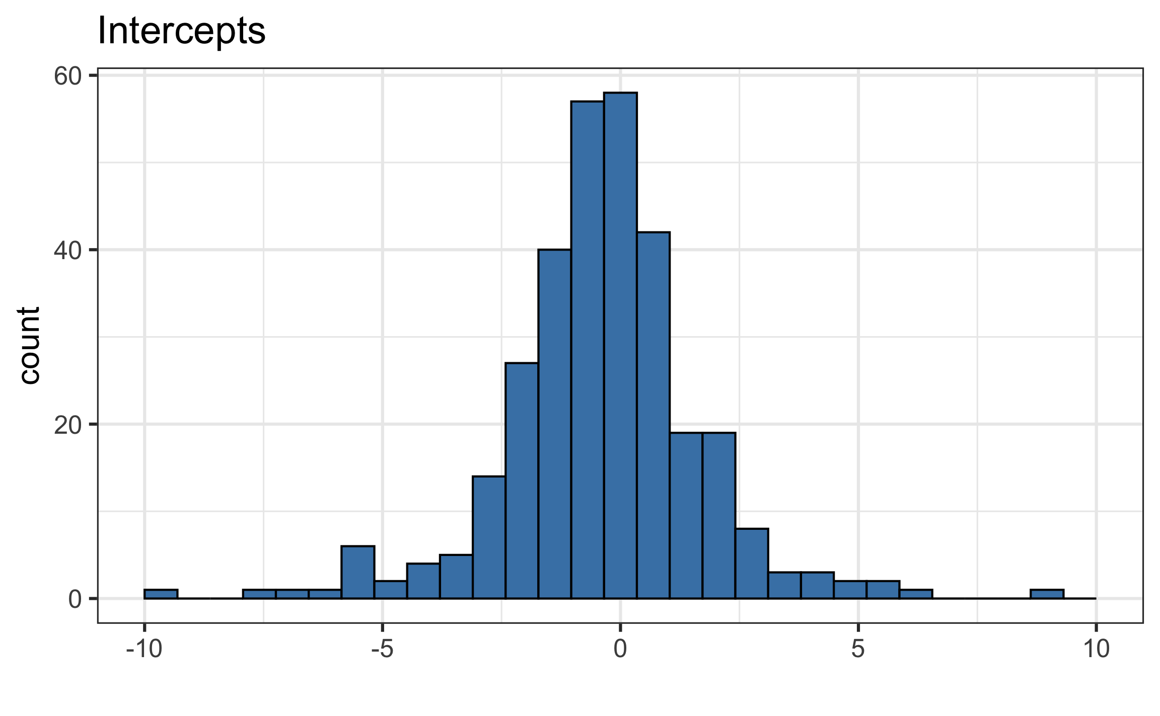
| alpha0 | sigma2_u |
|---|---|
| -0.301 | 128.858 |
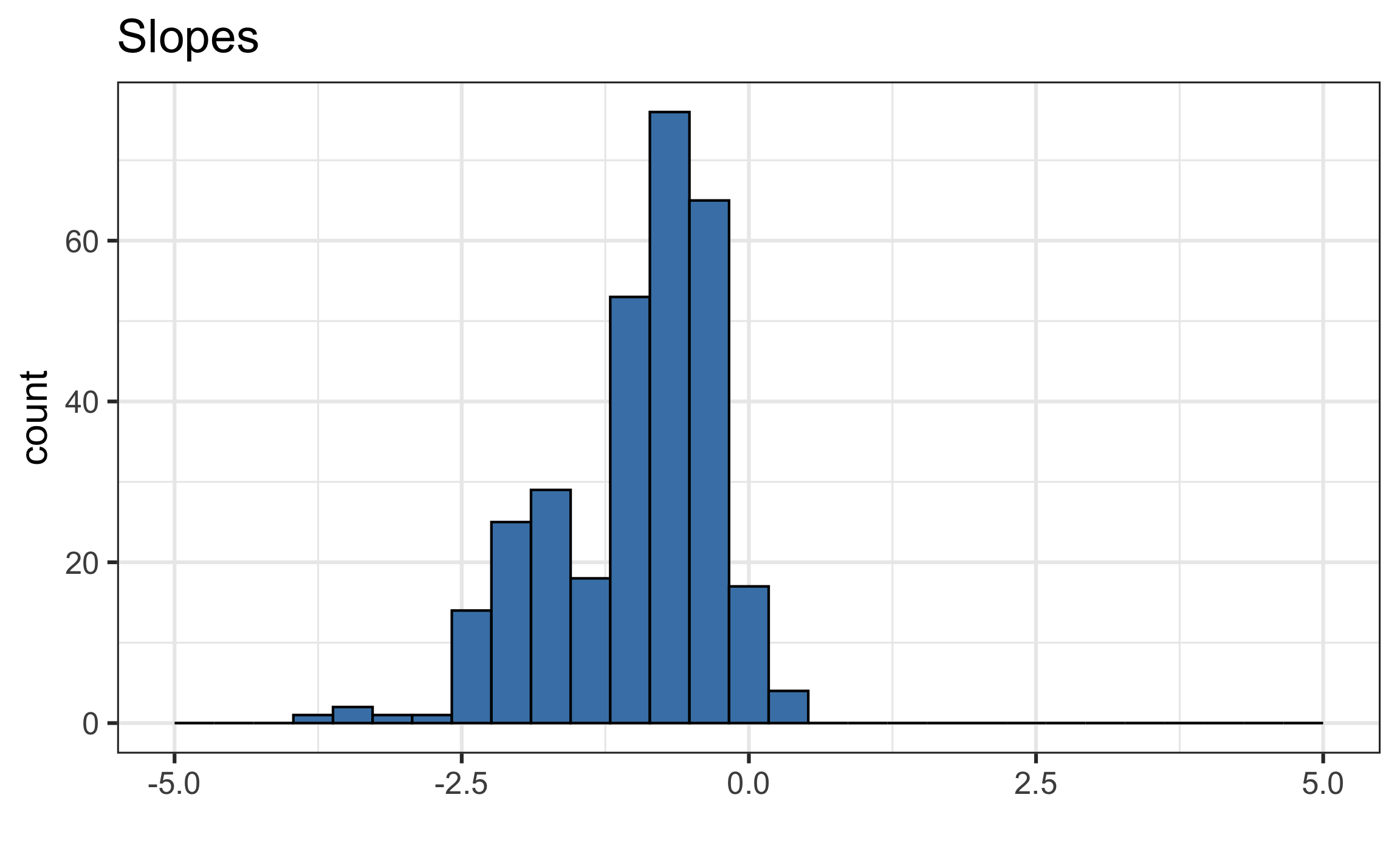
| beta0 | sigma2_v |
|---|---|
| -3.328 | 60.049 |
What do we learn from the distribution of the slopes and intercepts?
Consider number of fouls per game
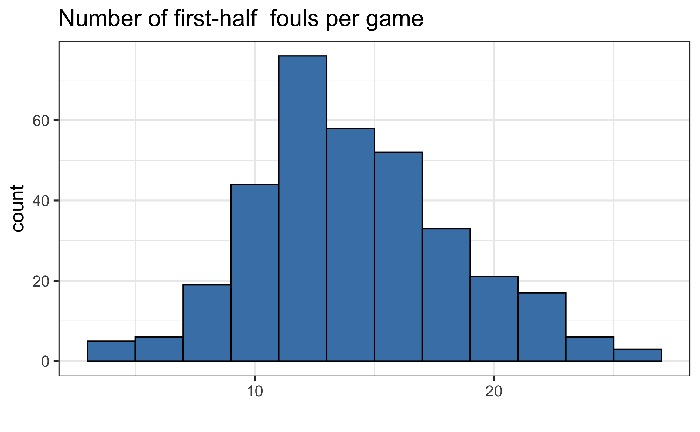
Warning
In the two-stage approach, games with 3 fouls are treated with equal weight as games with 20 + fouls
Unified multilevel model
Models by level
Level One models
\[\log\Big(\frac{p_{ij}}{1 - p_{ij}}\Big) = a_i + b_i ~ \text{foul.diff}_{ij}\] Level Two models
\[a_i = \alpha_0 + u_i\hspace{20mm} b_i = \beta_0 + v_i\]
\[\left[ \begin{array}{c} u_i \\ v_i \end{array} \right] \sim N \left( \left[ \begin{array}{c} 0 \\ 0 \end{array} \right], \left[ \begin{array}{cc} \sigma_u^{2} & \sigma_{uv} \\ \sigma_{uv} & \sigma_{v}^{2} \end{array} \right] \right)\]
Composite model
Composite model \[\log\Big(\frac{p_{ij}}{1 - p_{ij}}\Big) = \alpha_0 + \beta_0 ~ \text{foul.diff}_{ij} + [u_i + v_i ~ \text{foul.diff}_{ij}]\] \[\left[ \begin{array}{c} u_i \\ v_i \end{array} \right] \sim N \left( \left[ \begin{array}{c} 0 \\ 0 \end{array} \right], \left[ \begin{array}{cc} \sigma_u^{2} & \sigma_{uv} \\ \sigma_{uv} & \sigma_{v}^{2} \end{array} \right] \right)\]
Fit the model in R
Use the glmer function in the lme4 package to fit multilevel GLMs.
boundary (singular) fit: see help('isSingular')| effect | group | term | estimate | std.error | statistic | p.value |
|---|---|---|---|---|---|---|
| fixed | NA | (Intercept) | -0.157 | 0.046 | -3.382 | 0.001 |
| fixed | NA | foul.diff | -0.285 | 0.038 | -7.440 | 0.000 |
| ran_pars | game | sd__(Intercept) | 0.542 | NA | NA | NA |
| ran_pars | game | cor__(Intercept).foul.diff | -1.000 | NA | NA | NA |
| ran_pars | game | sd__foul.diff | 0.035 | NA | NA | NA |
Boundary constraints
Boundary constraints
The estimates of the parameters \(\alpha_0, \beta_0, \sigma_u, \sigma_v, \rho_{uv}\) are those that maximize the likelihood of observing the data
The fixed effects, e.g., \(\alpha_0\) and \(\beta_0\), can take any values, but the terms associated with the error terms are constrained to a set of “allowable” values
- \[\sigma_u \geq 0 \hspace{10mm} \sigma_v \geq 0 \hspace{10mm} -1 \leq \rho_{uv} \leq 1\]
Because of these boundaries, a “constrained” search is used to find the MLEs.
The error message
"## boundary (singular) fit", means the estimate of one or more terms was set at the maximum (or minimum) allowable value, not the value it would’ve been if an unconstrained search were allowable
Illustrating boundary constraints
Contour plots from a hypothetical likelihood \(L(\beta_0, \sigma^2)\)
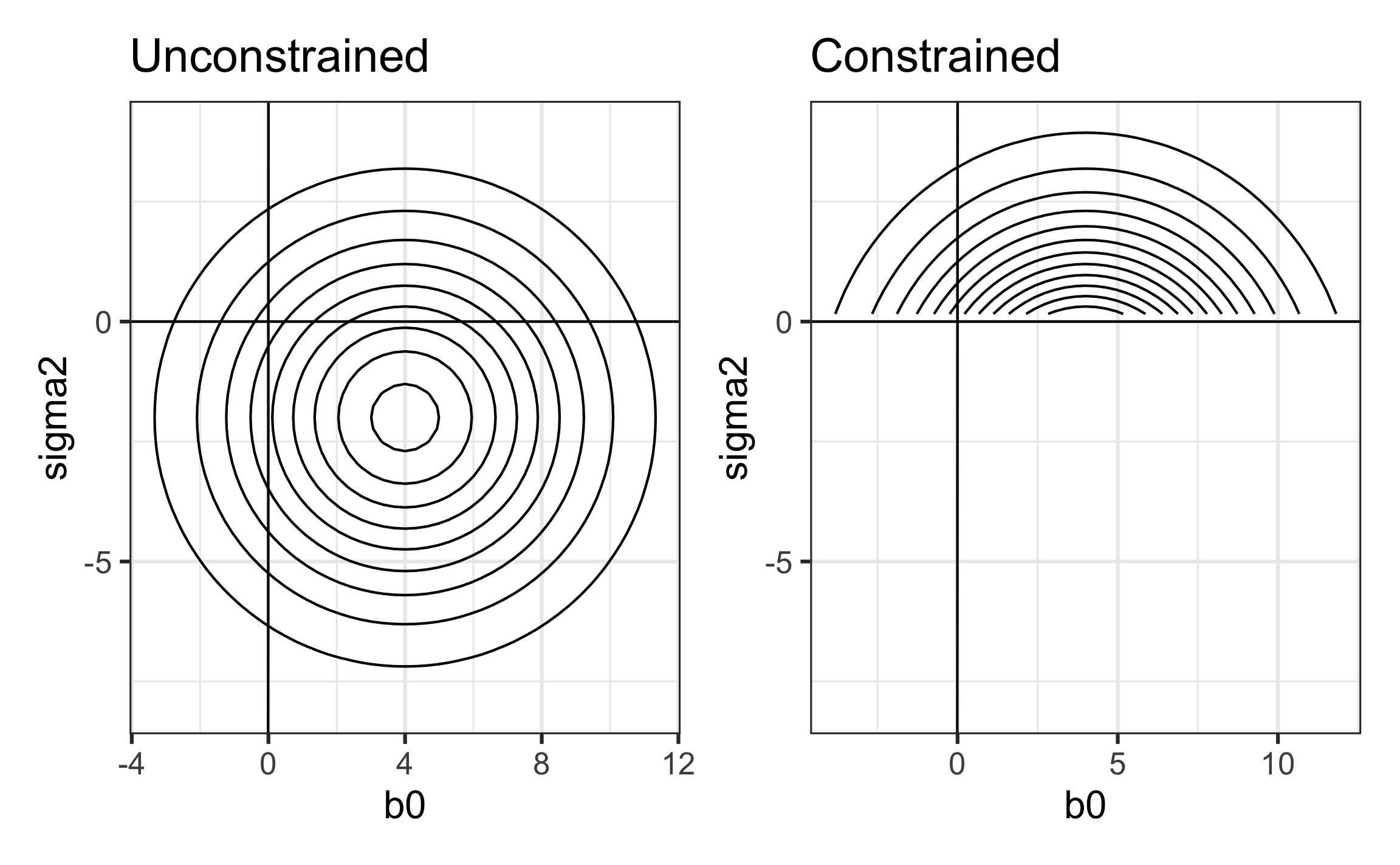
In the unconstrained search, the likelihood \(L(\beta_0, \sigma^2)\) is maximized at \(\hat{\beta}_0 = 4, \hat{\sigma}^2 = -2\)
In reality \(\sigma^2\) must be non-negative, so the search for the MLE is restricted to the region such that \(\sigma^2 \geq 0\).
The constrained likelihood is maximized at \(\hat{\beta}_0 = 4, \hat{\sigma}^2 = 0\)
Addressing boundary constraints
Address boundary constraints by reparameterizing the model
Remove variance and/or correlation terms estimated at the boundary
Reduce the number of parameters to be estimated by fixing the values of some parameters
Apply transformation to covariates, such as centering variables, standardizing variables, or changing units. Extreme values, outliers, or highly correlated covariates can sometimes cause issues with MLEs.
Is it OK to use model that faces boundary constraints?
Best to try to deal with boundary constraints, but you can sometimes leave the model as is if…
You’re not interested in estimating parameters with boundary issues
Removing the parameters does not impact conclusions about the variables of interest
Original model
| effect | group | term | estimate | std.error | statistic | p.value |
|---|---|---|---|---|---|---|
| fixed | NA | (Intercept) | -0.157 | 0.046 | -3.382 | 0.001 |
| fixed | NA | foul.diff | -0.285 | 0.038 | -7.440 | 0.000 |
| ran_pars | game | sd__(Intercept) | 0.542 | NA | NA | NA |
| ran_pars | game | cor__(Intercept).foul.diff | -1.000 | NA | NA | NA |
| ran_pars | game | sd__foul.diff | 0.035 | NA | NA | NA |
- Which term(s) should we remove to try to address boundary constraint?
- Refit the model with these terms removed. 3. Which model do you choose? Explain.
04:00
Interpret model coefficients
Interpret the following coefficients in the selected model (if applicable):
\(\hat{\alpha}_0\)
\(\hat{\beta}_0\)
\(\hat{\sigma}_u\)
\(\hat{\sigma}_v\)
\(\hat{\rho}_{uv}\)
Looking ahead
So far we’ve only considered random effects within a nested structure, but sometimes we may want to consider random effects that aren’t nested.
For example, we want to consider a random effect for the home team, but home team is not nested within game (since teams can be the home team for multiple games)
We will deal with this using crossed random effects
