library(tidyverse)
library(knitr)
library(lme4)
library(broom.mixed)
library(viridis)Lecture 20: Multilevel generalized linear models
basketball <- read_csv("data/basketball0910.csv")See Section 11.1: Multilevel generalized linear models for the full codebook.
Exploratory data analysis
Univariate EDA
Make a table or visualization of the distribution of the response variable,foul.home. What proportion of fouls are called on the home team?
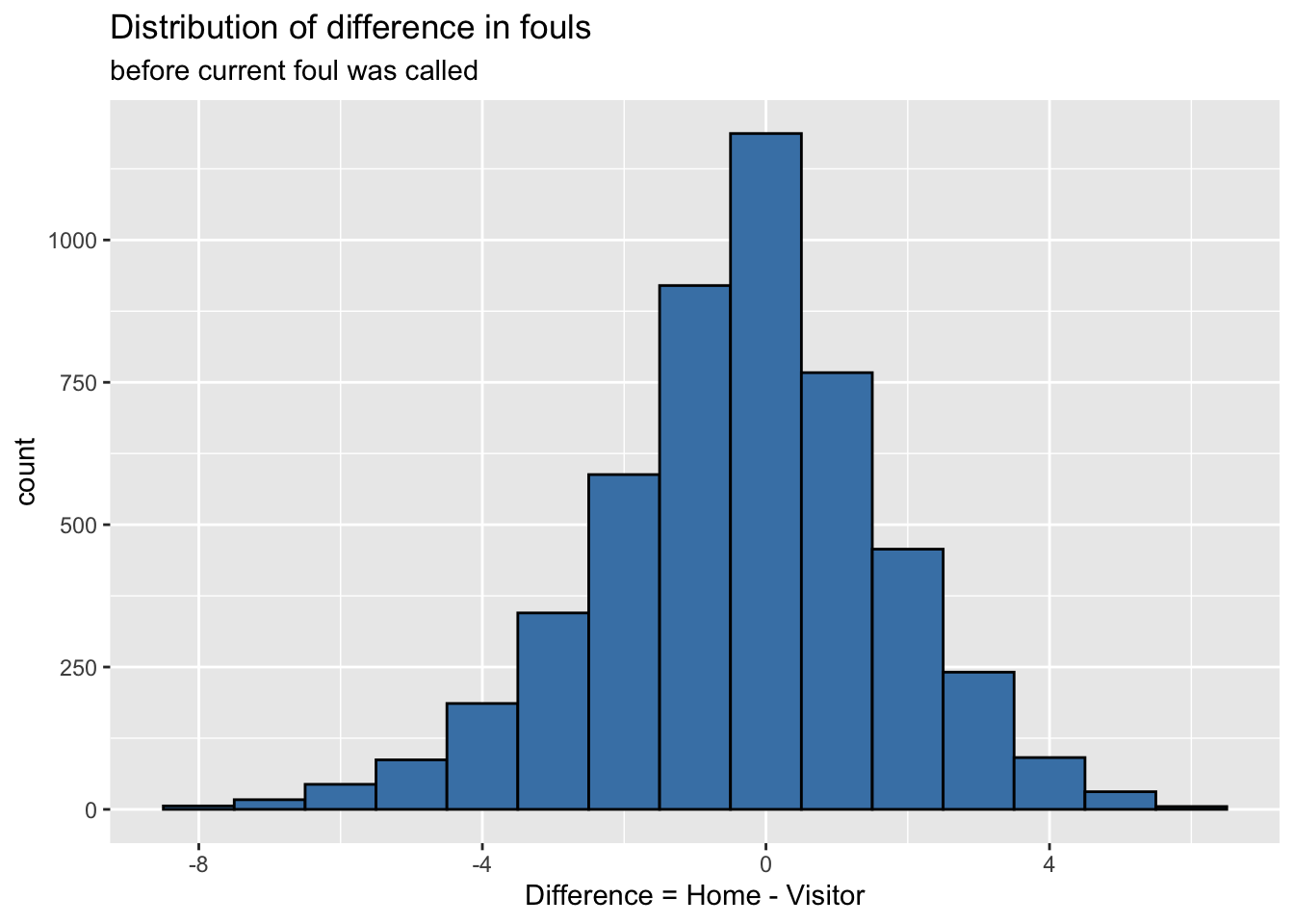
A histogram of the primary predictor of interest, foul.diff is below. Describe the distribution. Based on this, does it appear referees try to even out fouls called on the home and visiting teams?
ggplot(data = basketball, aes(x = foul.diff)) +
  geom_histogram(binwidth = 1, color = "black", fill = "steelblue") +
  labs(x = "Difference = Home - Visitor",
       title = "Distribution of difference in fouls",
       subtitle = "before current foul was called")
Below is the average total number of fouls in all games in which a given team was the home team.
basketball |>
  group_by(hometeam, game) |>
  summarise(total_fouls = sum(foul.home, foul.vis)) |>
  group_by(hometeam) |>
  summarise(avg_foul = sum(total_fouls) / n())
# A tibble: 39 × 2
hometeam avg_foul
<chr> <dbl>
1 BC 15.1
2 CIN 12.2
3 CLEM 15.5
4 CT 15
5 DEPAUL 13.4
6 DUKE 20
7 FLST 16.6
8 GATECH 17.5
9 GTOWN 13.8
10 IA 12.1
# ℹ 29 more rowsThe most total number fouls were called, on average, when which team was the home team? How many fouls were called on average?
The least total number fouls were called, on average, when which team was the home team? How many fouls were called on average?
Does this support including a random effect for home team in the model? Explain.
Bivariate EDA
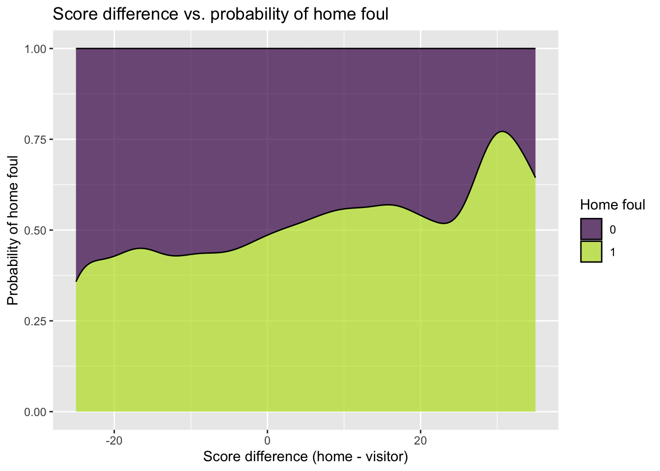
Below is a conditional density plot of score.diff, the score differential before the foul was called versus the response variable foul.home. Describe the relationship between score differential and the probability a foul called was on the home team.
ggplot(data = basketball, aes(x = score.diff, fill = factor(foul.home))) +
  geom_density(position = "fill", adjust = 2, alpha = 0.7) +
  labs(x = "Score difference (home - visitor)",
       y = "Probability of home foul",
       fill = "Home foul",
       title = "Score difference vs. probability of home foul") +
  scale_fill_viridis_d(end = 0.9)
Make a conditional density plot of foul.diff versus the response variable foul.home. Describe the relationship between foul differential and the probability a foul called was on the home team.
# conditional density plotMake an empirical logit plot of foul.diff versus the logit of foul.home. Based on this plot, is the logit link function appropriate to model this data?
# empirical logit Multilevel model
Original model
model1 <- glmer(foul.home ~ foul.diff + (foul.diff|game),
                data = basketball, family = binomial)
tidy(model1)
# A tibble: 5 × 7
effect group term estimate std.error statistic p.value
<chr> <chr> <chr> <dbl> <dbl> <dbl> <dbl>
1 fixed <NA> (Intercept) -0.157 0.0464 -3.38 7.19e- 4
2 fixed <NA> foul.diff -0.285 0.0383 -7.44 1.01e-13
3 ran_pars game sd__(Intercept) 0.542 NA NA NA
4 ran_pars game cor__(Intercept).foul.d… -1 NA NA NA
5 ran_pars game sd__foul.diff 0.0351 NA NA NA Reparameterize model
Which term(s) should we remove to try to address boundary constraint?
Refit the model with these terms removed. Call this model2.
# refit model Which model do you choose - model1 or model2? Explain.
Interpret coefficients
Interpret the applicable coefficients in the selected model:
\(\hat{\alpha}_0\):
\(\hat{\beta}_0\):
\(\hat{\sigma}_u\):
\(\hat{\sigma}_v\):
\(\hat{\rho}_{uv}\):
