STA 310 - Spring 2024 - Modeling data with three (or more) levels

Announcements

Quiz 04 - due March 28 at noon
- Covers readings and lectures March 4 - 20
- Longitudinal modeling, Chapter 9 of BMLR
Project 02
- Presentations April 3 during lecture
- Written report + GitHub repo due April 4 at 11:59pm
Final project - Round 1 submission (optional) due April 25

Topics

Write form of model for models with more than two levels
Interpret fixed and random effects at each level
See how three-level models are used in data analysis example

Note

The notes are based on Chapter 10 of Roback and Legler (2021) and Jones (1991) unless otherwise noted.

Data: Housing prices in Southampton

The data includes the price and characteristics for 918 houses sold between 1986 and 1991 in Southampton, England. The data were originally collected from a local real estate agency and were analyzed in Jones (1991). The primary variables of interest are

price: Sales price in thousands of £
Age: Age of the house
Bedrooms: Number of bedrooms
House Type: (semi-detached, detached, bungalow, terrace, flat)
Central heating: Whether house has central heating (0: yes, 1: no)
Garage: Number of garages (none, single, double)
Districts: one of 34 districts
Half-years: Half-year periods beginning the second half of 1986

Data structure

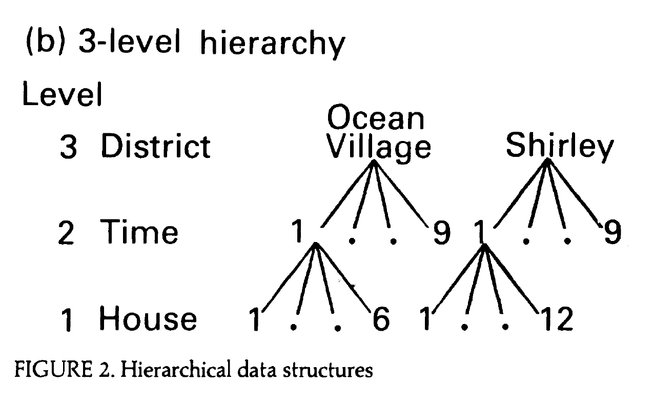
Portions of Figure 2b from Jones (1991)

Note

You can access the paper on Canvas.The paper uses different symbols to represent parameters than what is in the textbook. The slides will follow the textbook.

Unconditional means model

$\begin{aligned} Y_{i j k} = α_{0} + {\tilde{u}}_{i} + u_{i j} + ϵ_{i j k} \\ {\tilde{u}}_{i} \sim N (0, σ_{\tilde{u}}^{2}) u_{i j} \sim N (0, σ_{u}^{2}) ϵ_{i j k} \sim N (0, σ^{2}) \end{aligned}$

Level One (house within time)

$Y_{i j k} = a_{i j} + ϵ_{i j k}, ϵ_{i j k} \sim N (0, σ^{2})$

Level Two (time within district)

$a_{i j} = a_{i} + u_{i j}, u_{i j} \sim N (0, σ_{u}^{2})$

Level Three (district)

$a_{i} = α_{0} + {\tilde{u}}_{i}, {\tilde{u}}_{i} \sim N (0, σ_{\tilde{u}}^{2})$

Model A

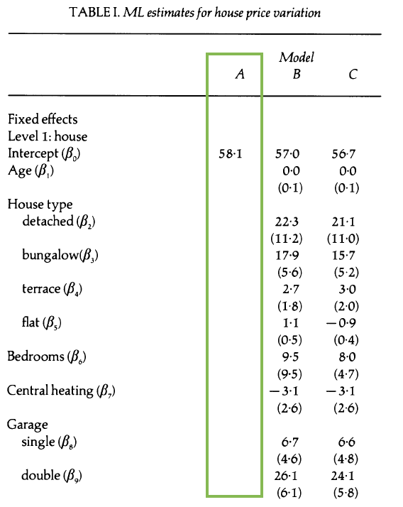
Interpret ${\hat{β}}_{0}$ (this is $α_{0}$ in our model notation)

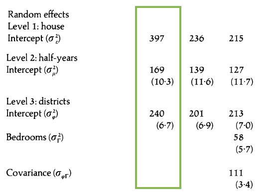
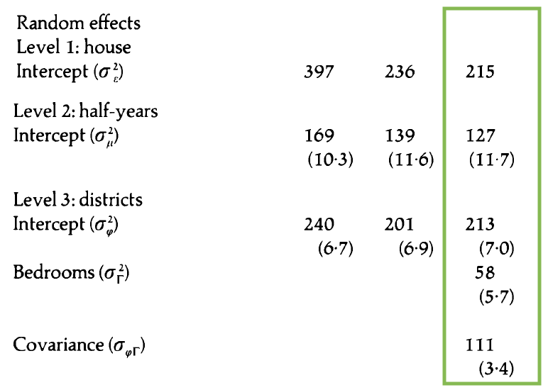
Model A: Random effects

About 29.8% of the variability in price is explained by differences between districts.
About 21% of the variability in price is explained by differences between time periods within the same district.
About 49.2% of the variability in price is explained by differences between houses in the same district sold in the same time period.

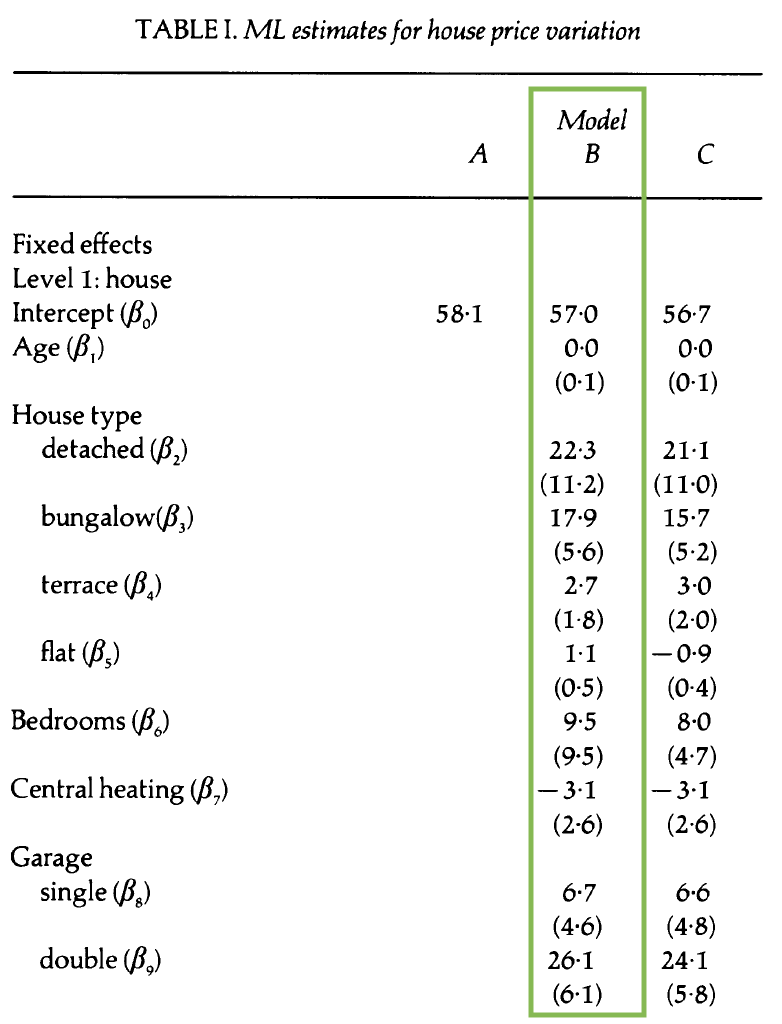
Model B: Covariates + random intercepts

Table 1 from Jones (1991)

Model B: Composite model

$\begin{aligned} Y_{i j k} & = α_{0} + β_{1} a g e_{i j k} + β_{2} d e t a c h e d_{i j k} + β_{3} b u n g a l o w_{i j k} \\ + β_{4} t e r r a c e_{i j k} + β_{5} f l a t_{i j k} + β_{6} b e d r o o m s_{i j k} + β_{7} h e a t i n g_{i j k} \\ + β_{8} s i n g l e_{i j k} + β_{9} d o u b l e_{i j k} + [{\tilde{u}}_{i} + u_{i j} + ϵ_{i j k}] \\ {\tilde{u}}_{i} \sim N (0, σ_{\tilde{u}}^{2}) u_{i j} \sim N (0, σ_{u}^{2}) ϵ_{i j k} \sim N (0, σ^{2}) \end{aligned}$

Write the Level One, Level Two, Level Three models.

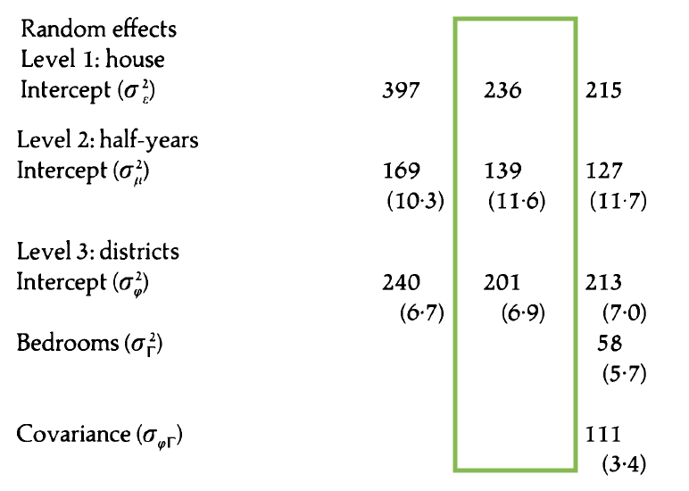
Model C: Additional random effect

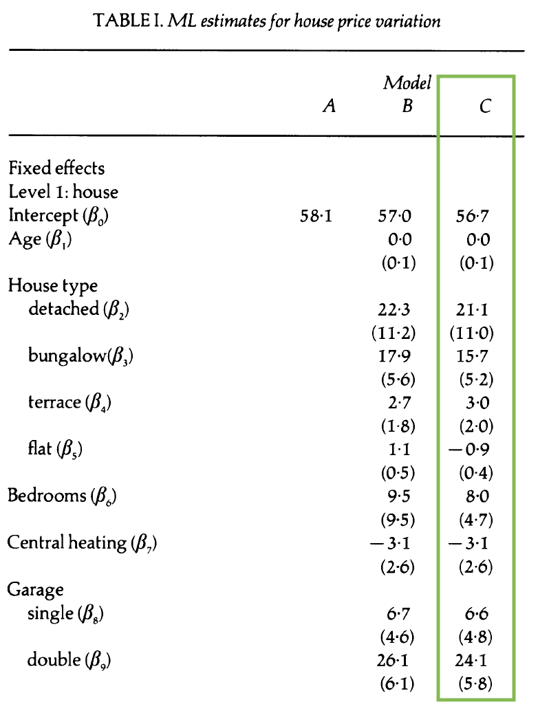
How does this model differ from Model B?
Write the composite model.
Write the Level One, Level Two, and Level Three models.

Visualizing price by district over time

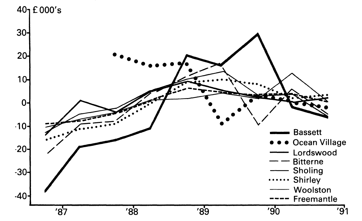
What do you observe from the plot?
What terms in the model can be understood from the plot?
How might you use this type of plot to support decisions you make in the analysis?

Price by district and bedrooms

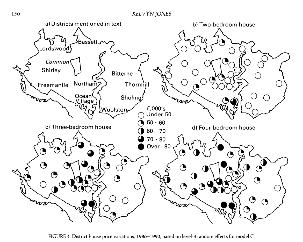
What do you observe from the plot?
What terms in the model can be understood from the plot?
How might you use this type of plot to support decisions you make in the analysis?

How does our understanding of the effect of bedrooms differ in this model compared to Model B?

Modeling data with three (or more) levels

Announcements

Topics

Data: Housing prices in Southampton

Data structure

Unconditional means model

Model A

Model A: Random effects

Model B: Covariates + random intercepts

Model B: Composite model

Model C: Additional random effect

Visualizing price by district over time

Price by district and bedrooms

Covariance structure of observations

Questions we want to answer

Calculating variance and covariance

Covariance structure under Model B

Variance and covariance derivations

References

![]()
Jones, Kelvyn. 1991. “Specifying and Estimating Multi-Level Models for Geographical Research.” Transactions of the Institute of British Geographers, 148–59.
Roback, Paul, and Julie Legler. 2021. Beyond multiple linear regression: applied generalized linear models and multilevel models in R. CRC Press.