Modeling data with three (or more) levels
Mar 25, 2024
Announcements
Quiz 04 - March 26 ~ 9am - March 28 at noon
Covers readings and lectures March 4 - 20
Longitudinal modeling, Chapter 9 of BMLR
Project 02
- Presentations April 3 during lecture
- Written report + GitHub repo due April 4 at 11:59pm
Final project - Round 1 submission (optional) due April 25
Topics
Write form of model for models with more than two levels
Interpret fixed and random effects at each level
See how three-level models are used in data analysis example
Sleep study
Data structure
Let’s look at the study about the effect of sleep on quality of life indicators. The data follow a multilevel structure with 3 levels
Level Three: Household
Level Two: Individual
- Level One: Wave
Outcomes of interest
We will focus on three of the outcomes:
Life satisfaction (
lfstat_OT): “represents a stable assessment of general feelings about life and indicates a long-term attitude”- Measured as response, ranging from 0 (extremely dissatisfied) to 10 (extremely satisfied), to the question “All things considered, how satisfied are you with your life as a whole?”
Wellbeing (
wellbe_OT): “captures a person’s emotional state and touches on their mental state”- Measured as average response, ranging from “at no time” to “all of the time”, to three items about how often in the last two weeks respondents “have been cheerful and in good spirits”, “have felt calm and relaxed”, and “have been active and vigorous”
Outcomes of interest
Happiness (
happy_OT): a person’s current positive emotional condition- Measured as response, ranging from 0 (extremely unhappy) to 10 (extremely happy), to the question “Taking all things together, how happy would you say you are?”
Sleep variables
sleep duration (
SDweek_OT)quality of sleep (
slequal_OT)social jetlag (
jetlag_OT)
Other covariates
- sex
- highest level of education attained (basic and secondary vocational, secondary with maturita, tertiary education)
- household income (divided into 6 categories)
- age
- employment status (employed, self-employed, unemployed, student, retired, on maternity leave)
- number of children below age 5 in the household
- wave (2018, 2019, 2020)
Conclusions
Recall the Modeling section in the lec-17 AE.
What are your conclusions about the effects of sleep on quality of life indicators?
Limitations
What are some potential limitations of this study?
Modeling data with three (or more) levels
Data: Housing prices in Southampton
The data includes the price and characteristics for 918 houses sold between 1986 and 1991 in Southampton, England. The data were originally collected from a local real estate agency and were analyzed in Jones (1991). The primary variables of interest are
- price: Sales price in thousands of £
- Age: Age of the house
- Bedrooms: Number of bedrooms
- House Type: (semi-detached, detached, bungalow, terrace, flat)
- Central heating: Whether house has central heating (0: yes, 1: no)
- Garage: Number of garages (none, single, double)
- Districts: one of 34 districts
- Half-years: Half-year periods beginning the second half of 1986
Data structure
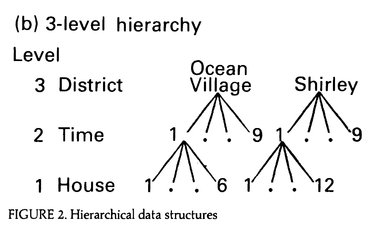
Portions of Figure 2b from Jones (1991)
Note
You can access the paper on Canvas.The paper uses different symbols to represent parameters than what is in the textbook. The slides will follow the textbook.
Unconditional means model
\[ Y_{ijk} = \alpha_0 + \tilde{u}_i + u_{ij} + \epsilon_{ijk} \]
Level One (house within time)
\(Y_{ijk} = a_{ij} + \epsilon_{ijk}, \hspace{10mm} \epsilon_{ijk} \sim N(0, \sigma^2)\)
Level Two (time within district)
\(a_{ij} = a_i + u_{ij}, \hspace{10mm} u_{ij} \sim N(0, \sigma^2_u)\)
Level Three (district)
\(a_{i} = \alpha_0 + \tilde{u}_{i}, \hspace{10mm} \tilde{u}_{i} \sim N(0, \sigma^2_{\tilde{u}})\)
Label the terms of the composite model
\(Y_{ijk}\): Price of house \(k\) in district \(i\) sold in time period \(j\)
\(\alpha_0\):
\(\epsilon_{ijk}\):
\(u_{ij}\)
\(\tilde{u}_i\):
\(\sigma\): Variance component describing house-to-house variability within a given time period
\(\sigma_{u}\): Variance component describing variability between time periods within a district
\(\sigma_{\tilde{u}}\): Variance component describing district-to-district variability
Model A
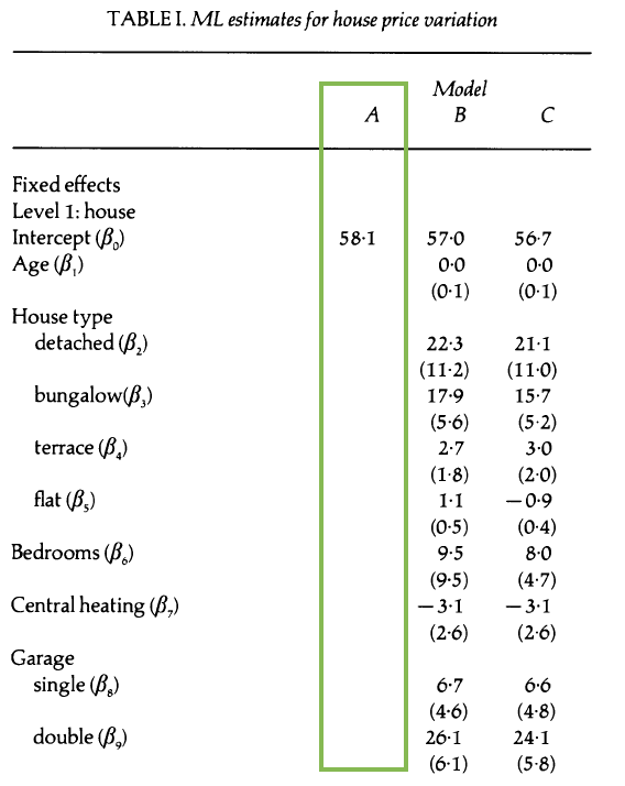
Interpret \(\hat{\beta}_0\) (this is \(\alpha_0\) in our model notation)
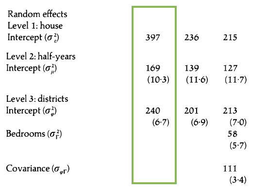
Model A: Random effects

- Calculate the intraclass correlation for time.
- Calculate the intraclass correlation coefficient for districts.
- Is there evidence the multilevel model structure is useful for this data?
Model B: Covariates + random intercepts
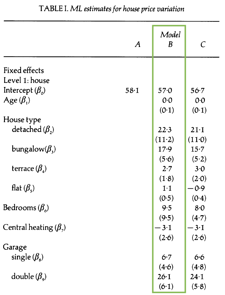
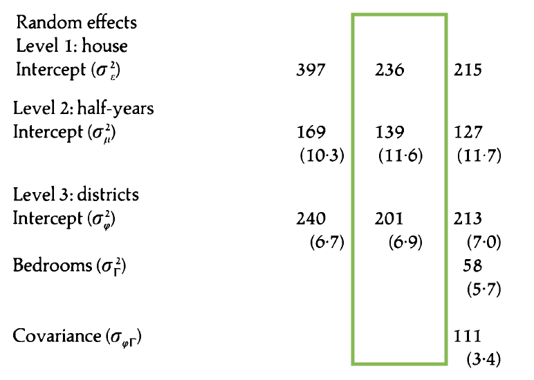
- Write the composite model.
- Which variables appear to have a statistically significant effect on price?
- Use this model to interpret the effect of a double garage on the price of houses in Southampton.
Model C: Additional random effect
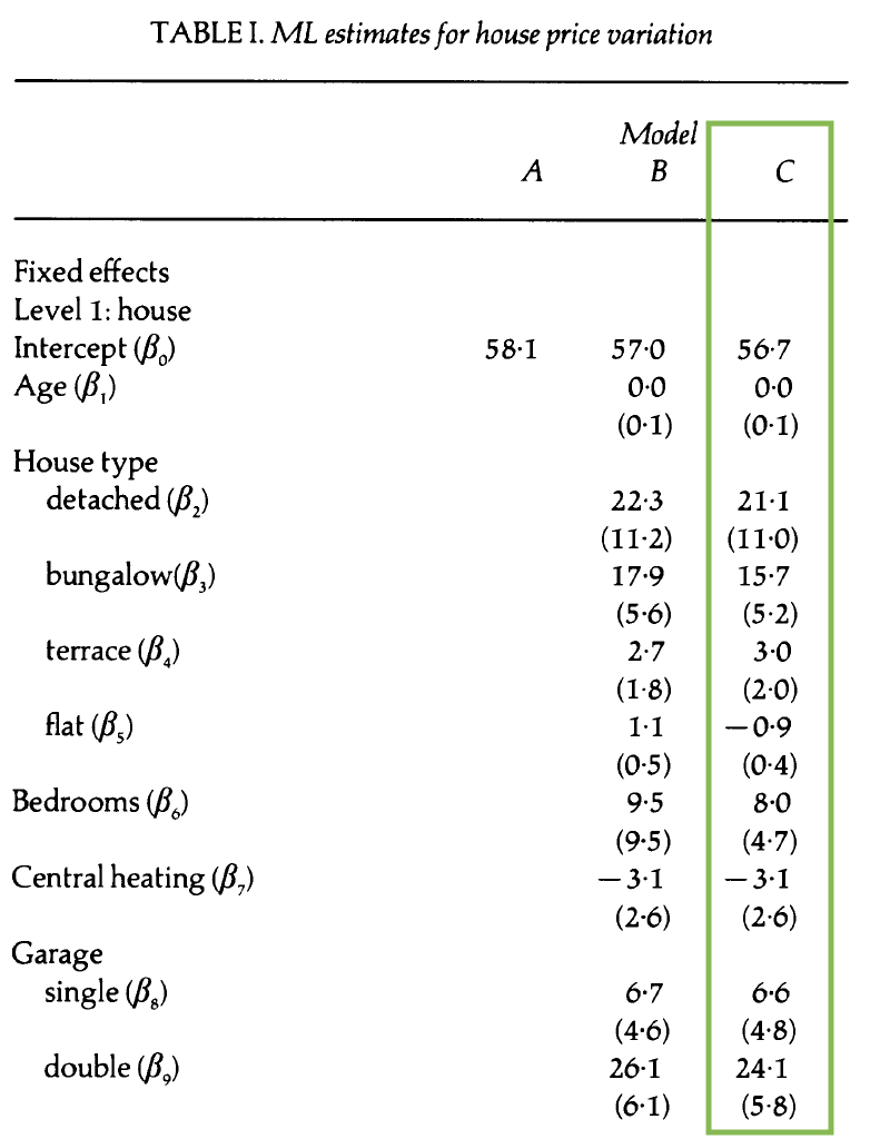
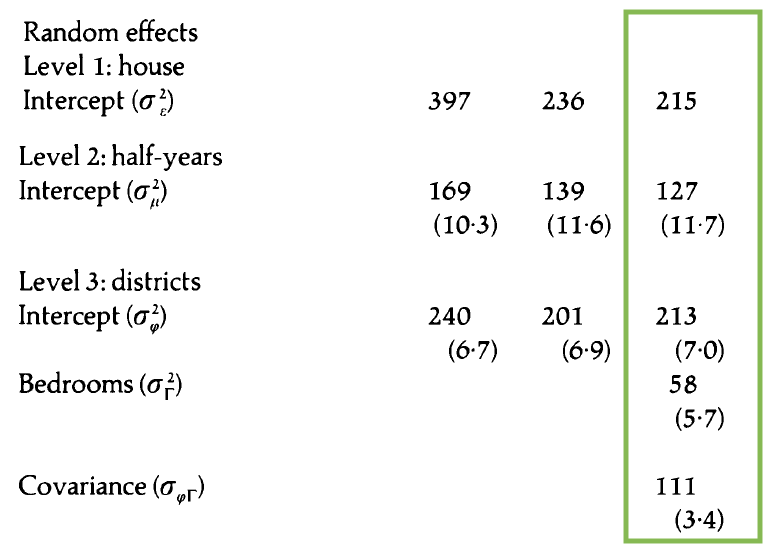
- How does this model differ from Model B?
- Write the composite model.
- Write the Level One, Level Two, and Level Three models.
Visualizing price by district over time
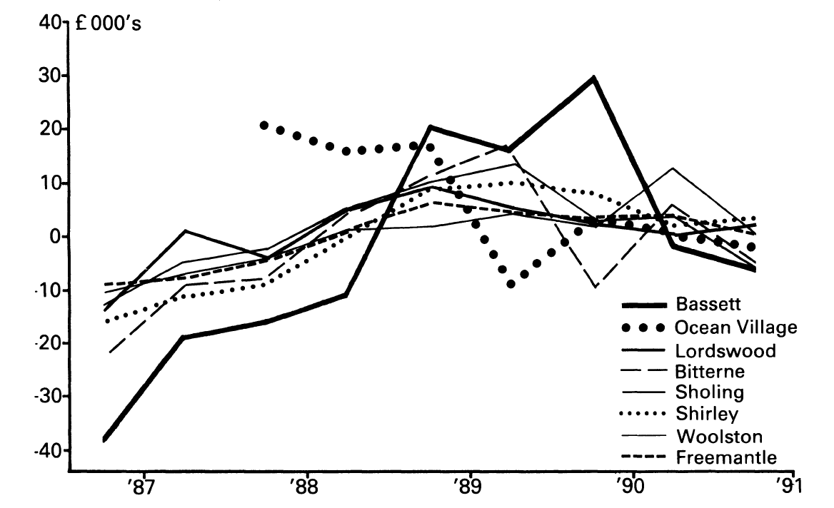
- What do you observe from the plot?
- What terms in the model can be understood from the plot?
- How might you use this type of plot to support decisions you make in the analysis?
Price by district and bedrooms
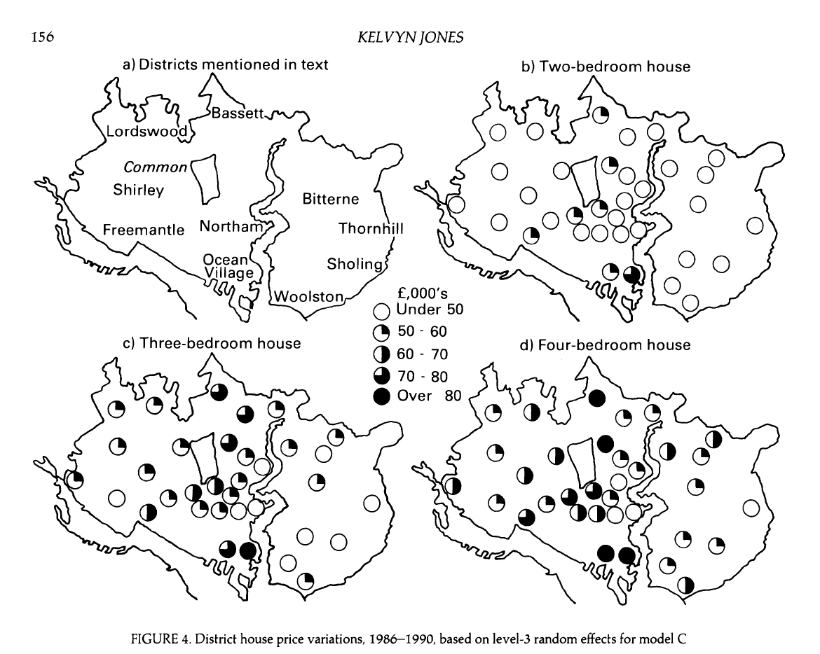
- What do you observe from the plot?
- What terms in the model can be understood from the plot?
- How might you use this type of plot to support decisions you make in the analysis?
How does our understanding of the effect of bedrooms differ in this model compared to Model B?
