| schoolName | year08 | urban | charter | schPctfree | MathAvgScore |
|---|---|---|---|---|---|
| RIPPLESIDE ELEMENTARY | 0 | 0 | 0 | 0.363 | 652.8 |
| RIPPLESIDE ELEMENTARY | 1 | 0 | 0 | 0.363 | 656.6 |
| RIPPLESIDE ELEMENTARY | 2 | 0 | 0 | 0.363 | 652.6 |
| RICHARD ALLEN MATH&SCIENCE ACADEMY | 0 | 1 | 1 | 0.545 | NA |
| RICHARD ALLEN MATH&SCIENCE ACADEMY | 1 | 1 | 1 | 0.545 | NA |
| RICHARD ALLEN MATH&SCIENCE ACADEMY | 2 | 1 | 1 | 0.545 | 631.2 |
Covariance structure of observations
Prof. Maria Tackett
Mar 18, 2024
Announcements
HW 04 due Wed, March 20 at 11:59pm
Project 02
- Draft report due Friday at noon
Topics
- Define the covariance structure of observations for a given model
- Understand how the covariance structure of observations differs from the covariance structure of error terms
- Calculate variance and covariance from model estimates
Data: Charter schools in MN
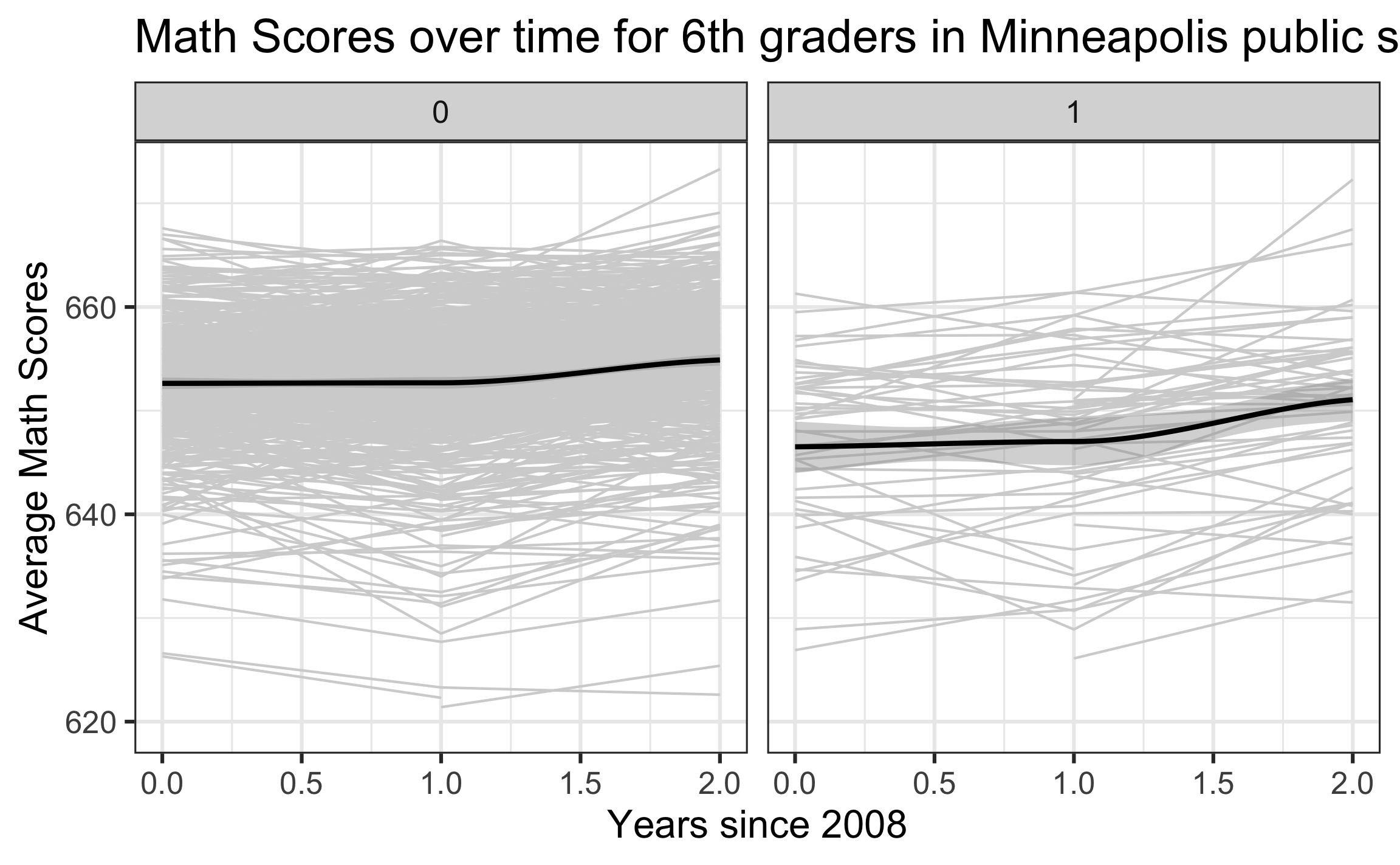
Today’s data set contains standardized test scores and demographic information for schools in Minneapolis, MN from 2008 to 2010. The data were collected by the Minnesota Department of Education. Understanding the effectiveness of charter schools is of particular interest, since they often incorporate unique methods of instruction and learning that differ from public schools.
MathAvgScore: Average MCA-II score for all 6th grade students in a school (response variable)urban: urban (1) or rural (0) location school locationcharter: charter school (1) or a non-charter public school (0)schPctfree: proportion of students who receive free or reduced lunches in a school (based on 2010 figures).year08: Years since 2008
Data
Exploratory data analysis
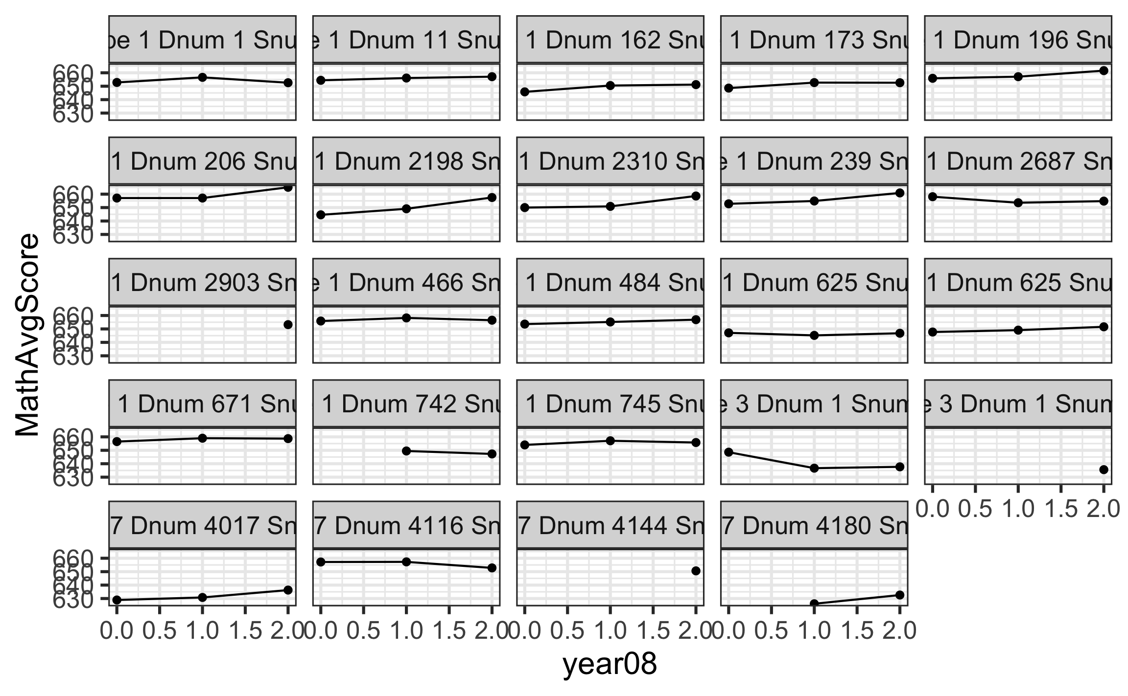
Exploratory data analysis
Model
We will use Model C1: Uncontrolled effects for school type.
\[ \begin{aligned} Y_{ij} &= \alpha_0 + \alpha_1Charter_i + \beta_0Year08_{ij} + \beta_1Charter_iYear08_{ij}\\&+ u_i + v_iYear08_{ij} + \epsilon_{ij} \\[8pt] &\epsilon_{ij} \sim N(0, \sigma^2) \hspace{15mm} \left[ \begin{array}{c} u_{i} \\ v_{i} \end{array} \right] \sim N \left( \left[ \begin{array}{c} 0 \\ 0 \end{array} \right], \left[ \begin{array}{cc} \sigma_{u}^{2} & \sigma_{uv} \\ \sigma_{uv} & \sigma_{v}^{2} \end{array} \right] \right) \end{aligned} \]
What we’ve done
So far we have discussed…
- the covariance structure between error terms at a given level, e.g. the distribution of between \(u_i\) and \(v_i\) from a Level Two model:
\[\left[ \begin{array}{c} u_{i} \\ v_{i} \end{array} \right] \sim N \left( \left[ \begin{array}{c} 0 \\ 0 \end{array} \right], \left[ \begin{array}{cc} \sigma_{u}^{2} & \sigma_{uv} \\ \sigma_{uv} & \sigma_{v}^{2} \end{array} \right] \right)\]
- how to use the intraclass correlation coefficient to get an idea of the average correlation between observations nested in the same Level Two group (school)
Questions we want to answer
Now we want to be able to answer more specific questions about the covariance (and correlation) structure of observations at different levels.
How does the variability in 2008 and 2010 scores from the same school compare?
What is the correlation between 2008 and 2009 scores from the same school? What is the correlation between 2009 and 2010 scores? 2008 and 2010?
Covariance structure
The covariance structure of the three time points (2008, 2009, 2010) for School \(i\) is
\[\small{Cov(\textbf{Y}_{i}) = \left[ \begin{array}{ccc} Var(Y_{i1}) & Cov(Y_{i1}, Y_{i2}) & Cov(Y_{i1}, Y_{i3})\\ Cov(Y_{i1}, Y_{i2}) & Var(Y_{i2})& Cov(Y_{i2}, Y_{i3}) \\ Cov(Y_{i1}, Y_{i3}) &Cov(Y_{i2}, Y_{i3}) & Var(Y_{i3})\\ \end{array} \right]}\]
Do you expect the covariances to be positive or negative? Why?
Covariance structure and error terms
Note that covariance structure of observations is not the same as the error structure at Level Two.
\[ Cov(\mathbf{Y}_i) \neq \left[ \begin{array}{c} u_{i} \\ v_{i} \end{array} \right] \sim N \left( \left[ \begin{array}{c} 0 \\ 0 \end{array} \right], \left[ \begin{array}{cc} \sigma_{u}^{2} & \sigma_{uv} \\ \sigma_{uv} & \sigma_{v}^{2} \end{array} \right] \right) \]
Calculating variance and covariance
Suppose \(Y_1 = a_1 X_1 + a_2 X_2 + a_3\) and \(Y_2 = b_1 X_1 + b_2 X_2 + b_3\), where \(X_1\) and \(X_2\) are random variables and \(a_i\) and \(b_i\) are constants for \(i = 1, 2, 3\). Then we know from probability theory that
\[{\small\begin{aligned}Var(Y_1) & = a^{2}_{1} Var(X_1) + a^{2}_{2} Var(X_2) + 2 a_1 a_2 Cov(X_1,X_2) \\[10pt] Cov(Y_1,Y_2) & = a_1 b_1 Var(X_1) + a_2 b_2 Var(X_2) + (a_1 b_2 + a_2 b_1) Cov(X_1,X_2)\end{aligned}}\]
Note
This extends beyond two random variables
We will use these properties to define the covariance structure of the observations in the model.
Variance and covariance for Model C
\[ \begin{aligned} &Var(Y_{ij}) = \sigma^2_u + t^2_{ij}\sigma^2_v + \sigma^2 + 2t_{ij}\sigma_{uv} \\ &Cov(Y_{ij}, Y_{ik}) = \sigma^2_u + t_{ij}t_{ik}\sigma^2_v + (t_{ij} + t_{ik})\sigma_{uv} \end{aligned} \]
where \(t_{ij}\) is the \(j^{th}\) time period for school \(i\).
Let’s see how these equations were derived.
Model estimates
Get the estimates for \(\rho\), \(\sigma\), \(\sigma_u\), and \(\sigma_v\) from the model output
model <- lmer(MathAvgScore ~ charter + year08 + charter:year08 +
                (year08|schoolid), data = charter)
tidy(model) |> kable(digits = 3)| effect | group | term | estimate | std.error | statistic |
|---|---|---|---|---|---|
| fixed | NA | (Intercept) | 652.058 | 0.284 | 2291.998 |
| fixed | NA | charter1 | -6.018 | 0.866 | -6.953 |
| fixed | NA | year08 | 1.197 | 0.094 | 12.698 |
| fixed | NA | charter1:year08 | 0.856 | 0.314 | 2.723 |
| ran_pars | schoolid | sd__(Intercept) | 5.986 | NA | NA |
| ran_pars | schoolid | cor__(Intercept).year08 | 0.880 | NA | NA |
| ran_pars | schoolid | sd__year08 | 0.362 | NA | NA |
| ran_pars | Residual | sd__Observation | 2.964 | NA | NA |
Estimated variances and covariances
Within-school variance for 2008 time point \((t_{i1} = 0)\)
\[ \begin{aligned} \hat{Var}(Y_{i1}) &= 5.986^2 + 0^2*0.362^2 + 2.964^2 \\ &+ 2*0*(0.880 *5.986*0.362) \\ & = \mathbf{44.617} \end{aligned} \]
Within-school covariance between 2008 and 2009 \((t_{i1} = 0, t_{i2} = 1)\)
\[ \begin{aligned} \hat{Cov}(Y_{i1}, Y_{i2}) &= 5.986^2 + 0 * 1 * 0.362^2 \\ &+ (0 + 1)(0.880 *5.986*0.362) \\ & = \mathbf{37.739} \end{aligned} \]
Estimated covariance structure
\[ \hat{Cov}(\mathbf{Y}) =\left[ \begin{array}{ccc} 44.62 & 37.74 & 39.65\\ 37.74 & 48.56& 41.81 \\ 39.65 &41.81 & 52.77\\ \end{array} \right]\]
Correlation between observations
\[Corr(Y_1, Y_2) = \frac{Cov(Y_1, Y_2)}{\sqrt{Var(Y_1)Var(Y_2)}}\]
\[ \begin{aligned} \hat{Corr}(Y_{i1}, Y_{i2}) &= \frac{37.74}{\sqrt{44.62 * 48.56}} \\ &= \mathbf{0.811} \end{aligned} \]
Write the within-school correlation matrix.
Notes on covariance and correlation matrices
Often observe higher correlation between observations that are closer in time.
- Is this the case in the MN schools data?
Often observe similar variability in all time points.
- Is this the case in the MN schools data?
Two-level model structure is very flexible. Note that the time points do not need to be evenly spaced nor does each school have to have the same number of measurements.
These concepts apply for all multilevel models not just those for longitudinal data.
Other multilevel data
Recall the data from Sadler and Miller (2010) on musicians and performance anxiety and the model
\[\begin{aligned}Y_{ij} &= (\alpha_0 + \alpha_1 ~ Orchestra_i + \beta_0 ~ LargeEnsemble_{ij} \\ &+ \beta_1 ~ Orchestra_i:LargeEnsemble_{ij})\\ &+ (u_i + v_i ~ LargeEnsemble_{ij} + \epsilon_{ij}) \\[8pt] &\epsilon_{ij} \sim N(0, \sigma^2) \hspace{15mm} \left[ \begin{array}{c} u_{i} \\ v_{i} \end{array} \right] \sim N \left( \left[ \begin{array}{c} 0 \\ 0 \end{array} \right], \left[ \begin{array}{cc} \sigma_{u}^{2} & \sigma_{uv} \\ \sigma_{uv} & \sigma_{v}^{2} \end{array} \right] \right)\end{aligned}\]
- Write the equation for \(Var(Y_{ij})\).
- Write the equation for \(Cov(Y_{ij}, Y_{ik})\).
Other multilevel data
\[ \begin{aligned} Var(Y_{ij}) & = \left\{ \begin{array}{ll} \sigma^{2} + \sigma_{u}^{2} & \mbox{if $\textrm{Large}_{ij}=0$} \\ \sigma^{2} + \sigma_{u}^{2} + \sigma_{v}^{2} + 2\sigma_{uv} & \mbox{if $\textrm{Large}_{ij}=1$} \end{array} \right.\end{aligned} \]
\[ \begin{aligned}Cov(Y_{ij},Y_{ik}) & = \left\{ \begin{array}{ll} \sigma_{u}^{2} & \mbox{if $\textrm{Large}_{ij}=\textrm{Large}_{ik}=0$} \\ \sigma_{u}^{2} + \sigma_{uv} & \mbox{if $\textrm{Large}_{ij}=0$, $\textrm{Large}_{ik}=1$ or vice versa} \\ \sigma_{u}^{2} + \sigma_{v}^{2} + 2\sigma_{uv} & \mbox{if $\textrm{Large}_{ij}=\textrm{Large}_{ik}=1$} \end{array} \right. \end{aligned} \]
Note
Every musician will have a unique covariance matrix depending on the number of performances and whether they are large or small ensemble.
Alternative covariance structures
The standard covariance structure calculated from the multilevel model is useful in most situations. Sometimes, however, there may be a different covariance structure that better fits the data. A few alternatives are
Unstructured: Every variance and covariance term for observations with each level is a separate parameter and is uniquely estimated. No patterns among variances or correlations are assumed. Very flexible but requires the estimation of many parameters.
Compound Symmetry: Assume variance is constant across all Level One observations and correlation is constant across all pairs of Level One observations. Restrictive but few parameters to estimate.
Alternative covariance structures
Autoregressive: Assume constant variance across all time points, but correlation reduces in a systematic way such that closer time points are more correlated than those further apart.
Toeplitz: Similar to autoregressive but there is no imposed structure on the decreased correlation for time periods further apart.
Heterogeneous variances: Allows for equal variances across time points. Requires additional parameters to be estimated to allow for the unequal variances.
Trying different covariance structures
There is generally little difference in estimates of fixed effects, and the impact on standard errors tends to be minimal.
If the primary analysis objective is inference and conclusions for fixed effects, it is often not worth spending too much time modeling different covariance structures.
If the analysis is also greatly interested in the random effects and estimated variance components, then the covariance structure can make a difference and it is worth modeling different covariance structures.
Tip
See “Fitting Linear Mixed Models in R” for details on R packages and code for multilevel models with a predetermined covariance structure.
References
Roback, Paul, and Julie Legler. 2021. Beyond multiple linear regression: applied generalized linear models and multilevel models in R. CRC Press.
Sadler, Michael E, and Christopher J Miller. 2010. “Performance Anxiety: A Longitudinal Study of the Roles of Personality and Experience in Musicians.” Social Psychological and Personality Science 1 (3): 280–87.