| schoolName | year08 | urban | charter | schPctfree | MathAvgScore |
|---|---|---|---|---|---|
| RIPPLESIDE ELEMENTARY | 0 | 0 | 0 | 0.363 | 652.8 |
| RIPPLESIDE ELEMENTARY | 1 | 0 | 0 | 0.363 | 656.6 |
| RIPPLESIDE ELEMENTARY | 2 | 0 | 0 | 0.363 | 652.6 |
| RICHARD ALLEN MATH&SCIENCE ACADEMY | 0 | 1 | 1 | 0.545 | NA |
| RICHARD ALLEN MATH&SCIENCE ACADEMY | 1 | 1 | 1 | 0.545 | NA |
| RICHARD ALLEN MATH&SCIENCE ACADEMY | 2 | 1 | 1 | 0.545 | 631.2 |
Modeling two-level longitudinal data
Inference for fixed and random effects
Mar 06, 2024
Announcements
Quiz 03 - due Thu, Mar 07 at noon
Covers readings and lectures in Feb 19 - 28 lectures
Correlated data, multilevel models
HW 04 - due Wed, Mar 20
- Released Thu, Mar 07 ~ 9am
Topics
- Inference for fixed and random effects
Modeling two-level longitudinal data
Data: Charter schools in MN
Today’s data set contains standardized test scores and demographic information for schools in Minneapolis, MN from 2008 to 2010. The data were collected by the Minnesota Department of Education. Understanding the effectiveness of charter schools is of particular interest, since they often incorporate unique methods of instruction and learning that differ from public schools.
MathAvgScore: Average MCA-II score for all 6th grade students in a school (response variable)urban: urban (1) or rural (0) location school locationcharter: charter school (1) or a non-charter public school (0)schPctfree: proportion of students who receive free or reduced lunches in a school (based on 2010 figures).year08: Years since 2008
Data
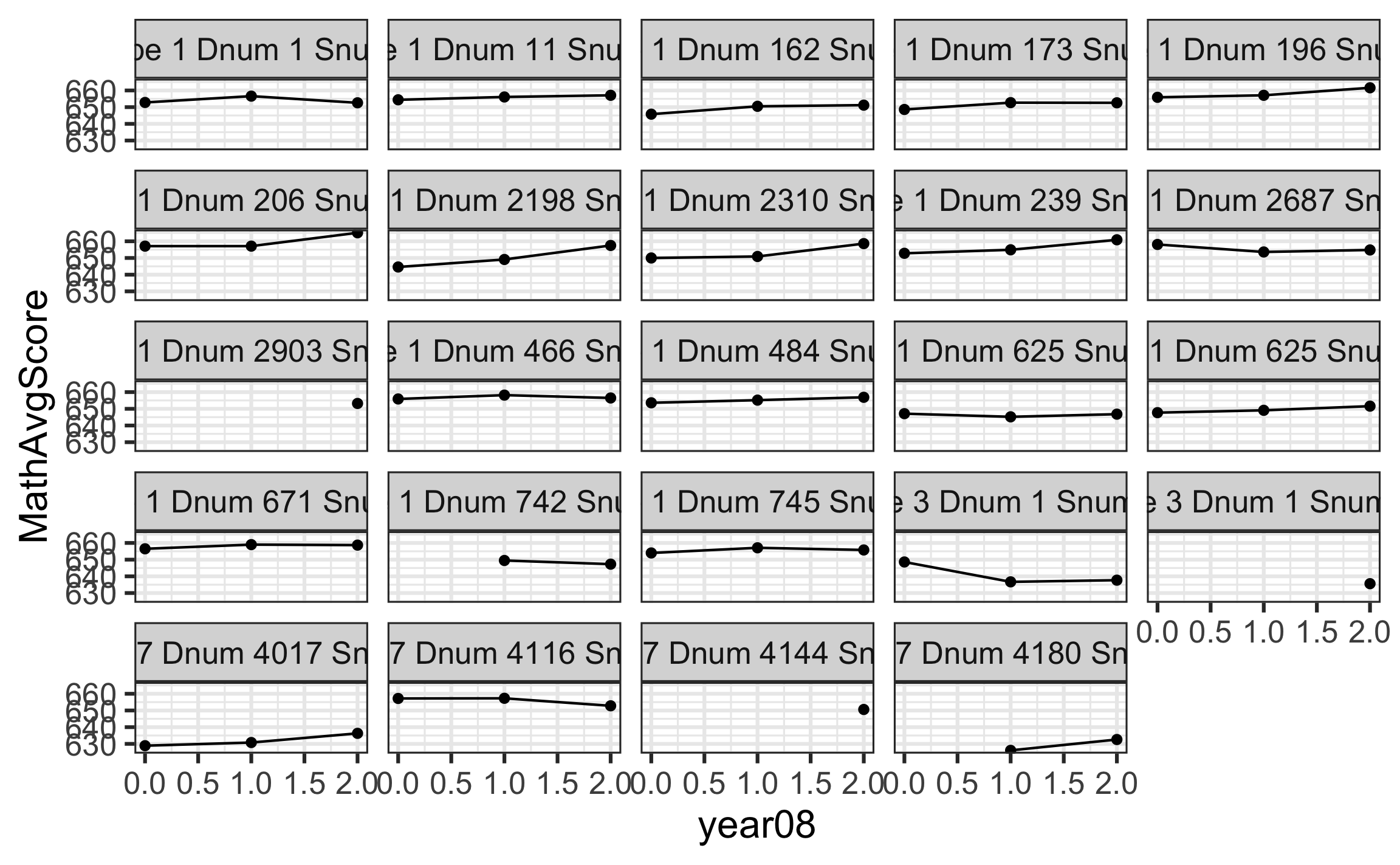
Closer look at missing data pattern
| MathAvgScore0_miss | MathAvgScore1_miss | MathAvgScore2_miss | n |
|---|---|---|---|
| 0 | 0 | 0 | 540 |
| 0 | 0 | 1 | 6 |
| 0 | 1 | 0 | 4 |
| 0 | 1 | 1 | 7 |
| 1 | 0 | 0 | 25 |
| 1 | 0 | 1 | 1 |
| 1 | 1 | 0 | 35 |
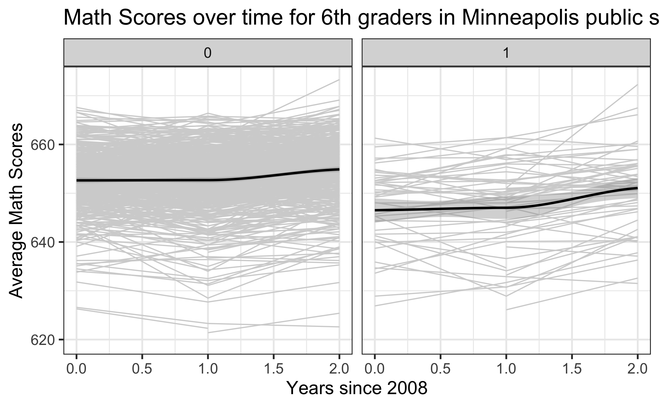
Exploratory data analysis

Exploratory data analysis

Unconditional means model
Start with the unconditional means model, a model with no covariates at any level. This is also called the random intercepts model.
Level One : \(Y_{ij} = a_{i} + \epsilon_{ij}, \hspace{5mm} \epsilon_{ij} \sim N(0, \sigma^2)\)
Level Two: \(a_i = \alpha_0 + u_i, \hspace{5mm} u_{i} \sim N(0, \sigma^2_u)\)
Unconditional growth model
A next step in the model building is the unconditional growth model, a model with Level One predictors but no Level Two predictors.
Level One
\[ Y_{ij} = a_i + b_iYear08_{ij} + \epsilon_{ij}, \hspace{8mm} \epsilon_{ij} \sim N(0, \sigma^2) \]
Level Two:
\[ \begin{aligned} &a_i = \alpha_0 + u_i \hspace{20mm} b_i = \beta_0 + v_i \\ &\left[ \begin{array}{c} u_{i} \\ v_{i} \end{array} \right] \sim N \left( \left[ \begin{array}{c} 0 \\ 0 \end{array} \right], \left[ \begin{array}{cc} \sigma_{u}^{2} & \sigma_{uv} \\ \sigma_{uv} & \sigma_{v}^{2} \end{array} \right] \right) \end{aligned} \]
Pseudo \(R^2\)
We can use Pseudo R2 to explain changes in variance components between two models
Note: This should only be used when the definition of the variance component is the same between the two models
\[\text{Pseudo }R^2 = \frac{\hat{\sigma}^2(\text{Model 1}) - \hat{\sigma}^2(\text{Model 2})}{\hat{\sigma}^2(\text{Model 1})}\]
We found that 17% of within-school variability in test scores by a change in scores over time.
Model with school-level covariates
Fit a model with school-level covariates that takes the following form:
Level One
\[\begin{equation*} Y_{ij}= a_{i} + b_{i}Year08_{ij} + \epsilon_{ij} \hspace{10mm} \epsilon_{ij} \sim N(0, \sigma^2) \end{equation*}\]Level Two
\[\begin{align*} a_{i} & = \alpha_{0} + \alpha_{1}charter_i + \alpha_{2}urban_i + \alpha_{3}schpctfree_i + u_{i} \\ b_{i} & = \beta_{0} + \beta_{1}charter_i + \beta_{2}urban_i + v_{i} \\[10pt] &\left[ \begin{array}{c} u_{i} \\ v_{i} \end{array} \right] \sim N \left( \left[ \begin{array}{c} 0 \\ 0 \end{array} \right], \left[ \begin{array}{cc} \sigma_{u}^{2} & \sigma_{uv} \\ \sigma_{uv} & \sigma_{v}^{2} \end{array} \right] \right) \end{align*}\]Model with school-level covariates
- Fit the model in R.
- Use the model to describe how the average math scores differed between charter and non-charter schools.
Consider a simpler model
Level One
\[\begin{equation*} Y_{ij}= a_{i} + b_{i}Year08_{ij} + \epsilon_{ij} \hspace{10mm} \epsilon_{ij} \sim N(0, \sigma^2) \end{equation*}\]Level Two
\[\begin{align*} a_{i} & = \alpha_{0} + \alpha_{1}charter_i + \alpha_{2}urban_i + \alpha_{3}schpctfree_i + u_{i} \hspace{10mm} u_i \sim N(0, \sigma_u^2) \\[8pt] b_{i} & = \beta_{0} + \beta_{1}charter_i + \beta_{2}urban_i \end{align*}\]In this model, the effect of year is the same for all schools with a given combination of charter and urban
Full and reduced models
Likelihood ratio test
| npar | AIC | BIC | logLik | deviance | Chisq | Df | Pr(>Chisq) | |
|---|---|---|---|---|---|---|---|---|
| reduced_model | 9 | 9952.992 | 10002.11 | -4967.496 | 9934.992 | NA | NA | NA |
| full_model | 11 | 9953.793 | 10013.83 | -4965.897 | 9931.793 | 3.199 | 2 | 0.202 |
\(\chi^2\) test is conservative, i.e., the p-values are larger than they should be, when testing random effects at the boundary ( e.g., \(\sigma_v^2 = 0\)) or those with bounded ranges (e.g., \(\rho_{uv}\) )
If you observe small p-values, you can feel relatively certain the tested effects are statistically significant
Use bootstrap methods to calculate confidence intervals or obtain more accurate p-values for LRT
Bootstrapping
Bootstrapping is from the phrase “pulling oneself up by one’s bootstraps”
Accomplishing a difficult task without any outside help
Task: conduct inference for model parameters (fixed and random effects) using only the sample data
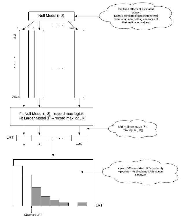
Parametric bootstrap for LRT
1️⃣ Fit the null (reduced) model to obtain the fixed effects and variance components (parametric part).
2️⃣ Use the estimated fixed effects and variance components to generate a new set of response values with the same sample size and associated covariates for each observation as the original data (bootstrap part).
3️⃣ Fit the full and null models to the newly generated data.
4️⃣ Compute the likelihood test statistic comparing the models from the previous step.
5️⃣ Repeat steps 2 - 4 many times (~ 1000).
Parametric bootstrap for LRT

Figure 9.19 in BMLR
Bootstrap CI
Use the confint function to calculate (parametric) bootstrapped confidence intervals to conduct inference on the fixed and random effects
| 2.5 % | 97.5 % | |
|---|---|---|
| sd_(Intercept)|schoolid | 4.0127 | 4.7203 |
| cor_year08.(Intercept)|schoolid | -0.2755 | 1.0000 |
| sd_year08|schoolid | 0.0384 | 0.9191 |
| sigma | 2.7839 | 3.0873 |
| (Intercept) | 659.3502 | 661.4273 |
| charter1 | -4.4390 | -1.5448 |
| urban1 | -2.0170 | -0.2651 |
| schPctfree | -19.3348 | -16.0699 |
| year08 | 1.2239 | 1.8147 |
| charter1:year08 | 0.4337 | 1.6641 |
| urban1:year08 | -0.9597 | -0.1922 |
Bootstrap CI
| 2.5 % | 97.5 % | |
|---|---|---|
| sd_(Intercept)|schoolid | 4.0127 | 4.7203 |
| cor_year08.(Intercept)|schoolid | -0.2755 | 1.0000 |
| sd_year08|schoolid | 0.0384 | 0.9191 |
| sigma | 2.7839 | 3.0873 |
| (Intercept) | 659.3502 | 661.4273 |
| charter1 | -4.4390 | -1.5448 |
| urban1 | -2.0170 | -0.2651 |
| schPctfree | -19.3348 | -16.0699 |
| year08 | 1.2239 | 1.8147 |
| charter1:year08 | 0.4337 | 1.6641 |
| urban1:year08 | -0.9597 | -0.1922 |
Would you keep \(\sigma_{v}\) or \(\rho_{uv}\) in the model?
Inference for fixed effects
The output for multilevel models do not contain p-values for the coefficients of fixed effects
The exact distribution of the test statistic under the null hypothesis (no fixed effect) is unknown, because the exact degrees of freedom are unknown
- Finding suitable approximations is an area of ongoing research
We can use likelihood ratio test with an approximate \(\chi^2\) distribution to test fixed effects
- Some research suggests the p-values are too low but approximations are generally pretty good
- Can also calculate the p-values using parametric bootstrap approach (can be computationally intensive)
Methods to conduct inference for individual estimates
- Use the t-value \(\big(\frac{estimate}{std.error}\big)\) in the model output for fixed effects
- General rule: Coefficients with |t-value| > 2 considered to be statistically significant, i.e., different from 0
- Likelihood ratio tests for fixed effects
- Calculate confidence intervals using parametric bootstrapping for fixed effects and variance components
Summary: Model comparisons
Methods to compare models with different fixed effects
- AIC or BIC
- Parametric bootstrap confidence intervals
- Likelihood ratio tests based on \(\chi^2\) distribution
- Likelihood ratio test based on parametric bootstrapped p-values (see Section 9.6.4 for more detail)
Methods to compare models with different variance components
- AIC or BIC
- Parametric bootstrap confidence intervals
- Likelihood ratio test based on parametric bootstrapped p-values (see Section 9.6.4 for more detail)
