| id | diary | large_ensemble | mpqnem | orchestra |
|---|---|---|---|---|
| 1 | 1 | 0 | 16 | 0 |
| 1 | 2 | 1 | 16 | 0 |
| 1 | 3 | 1 | 16 | 0 |
| 43 | 1 | 0 | 17 | 0 |
| 43 | 2 | 0 | 17 | 0 |
| 43 | 3 | 0 | 17 | 0 |
Multilevel models
Variance components + model fitting
Feb 26, 2024
Announcements
HW 03 released tomorrow due Wed, Feb 28 at 11:59pm
- See Slack for tips from Hun
Topics
Write multilevel model, including assumptions about variance components
- In by-level and composite forms
Fit and interpret multilevel models
Data: Music performance anxiety
Today’s data come from the study by Sadler and Miller (2010) of the emotional state of musicians before performances. The data set contains information collected from 37 undergraduate music majors who completed the Positive Affect Negative Affect Schedule (PANAS), an instrument produces a measure of anxiety (negative affect) and a measure of happiness (positive affect). This analysis will focus on negative affect as a measure of performance anxiety.
The primary variables we’ll use are
id: unique musician identification numberna: negative affect score on PANAS (the response variable)perform_type: type of performance (Solo, Large Ensemble, Small Ensemble)instrument: type of instrument (Voice, Orchestral, Piano)
Look at data
- What are the Level One and Level Two observational units?
- What variables are measured at each level?
Fitting the model
Questions we want to answer
What is the association between performance type (large ensemble or not) and performance anxiety? Does the association differ based on instrument type (orchestral or not)?
Initial modeling approach
Step 1. Fit a separate model for each musician understand the association between performance type (Level One models) and anxiety.
Step 2 . fit a system of Level Two models to predict the fitted coefficients in the Level One model for each subject based on instrument type (Level Two model).
Level One model
We’ll start with the Level One model to understand the association between performance type and performance anxiety for the \(i^{th}\) musician and the \(j^{th}\) performance \[na_{ij} = a_i + b_i ~ LargeEnsemble_{ij} + \epsilon_{ij}, \hspace{5mm} \epsilon_{ij} \sim N(0,\sigma^2)\]
For now, estimate \(a_i\) and \(b_i\) using least-squares regression.
Example Level One model
Below is data for id #22
# A tibble: 15 × 5
      id diary perform_type   instrument               na
   <dbl> <dbl> <chr>          <chr>                 <dbl>
 1    22     1 Solo           orchestral instrument    24
 2    22     2 Large Ensemble orchestral instrument    21
 3    22     3 Large Ensemble orchestral instrument    14
 4    22     4 Large Ensemble orchestral instrument    15
 5    22     5 Large Ensemble orchestral instrument    10
 6    22     6 Solo           orchestral instrument    24
 7    22     7 Solo           orchestral instrument    24
 8    22     8 Solo           orchestral instrument    16
 9    22     9 Small Ensemble orchestral instrument    34
10    22    10 Large Ensemble orchestral instrument    22
11    22    11 Large Ensemble orchestral instrument    19
12    22    12 Large Ensemble orchestral instrument    18
13    22    13 Large Ensemble orchestral instrument    12
14    22    14 Large Ensemble orchestral instrument    19
15    22    15 Solo           orchestral instrument    25
Level One model
| term | estimate | std.error | statistic | p.value |
|---|---|---|---|---|
| (Intercept) | 24.500 | 1.96 | 12.503 | 0.000 |
| large_ensemble1 | -7.833 | 2.53 | -3.097 | 0.009 |
Repeat for all 37 musicians.
Level One models
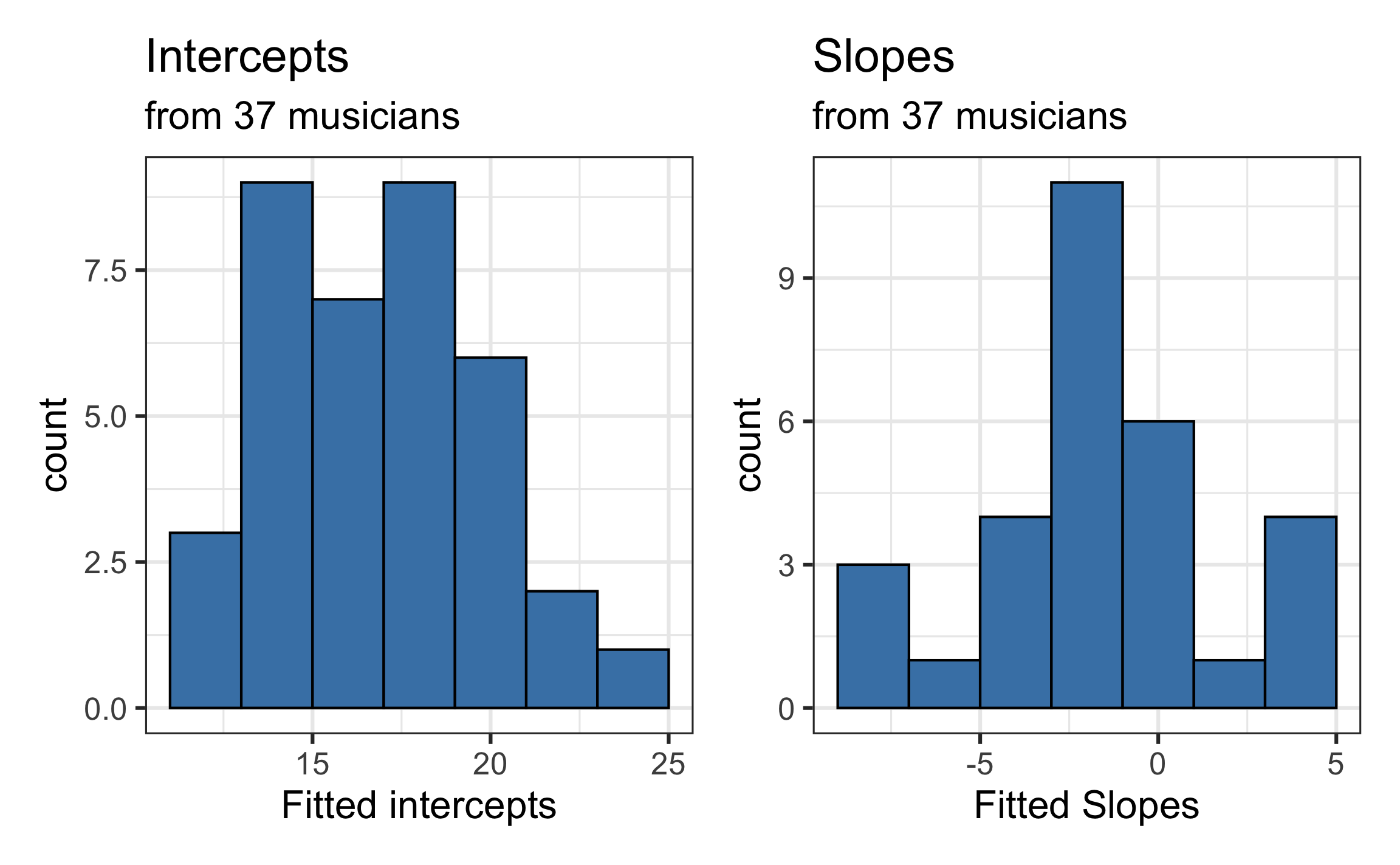
Recreated from BMLR Figure 8.9
Now let’s consider if there is an association between the estimated slopes, estimated intercepts, and the type of instrument
Level Two Model
The slope and intercept for the \(i^{th}\) musician can be modeled as \[\begin{aligned}&a_i = \alpha_0 + \alpha_1 ~ Orchestra_i + u_i \\ &b_i = \beta_0 + \beta_1 ~ Orchestra_i + v_i\end{aligned}\]
Note the response variable in the Level Two models are not observed outcomes but the (fitted) slope and intercept from each musician
Estimated coefficients by instrument
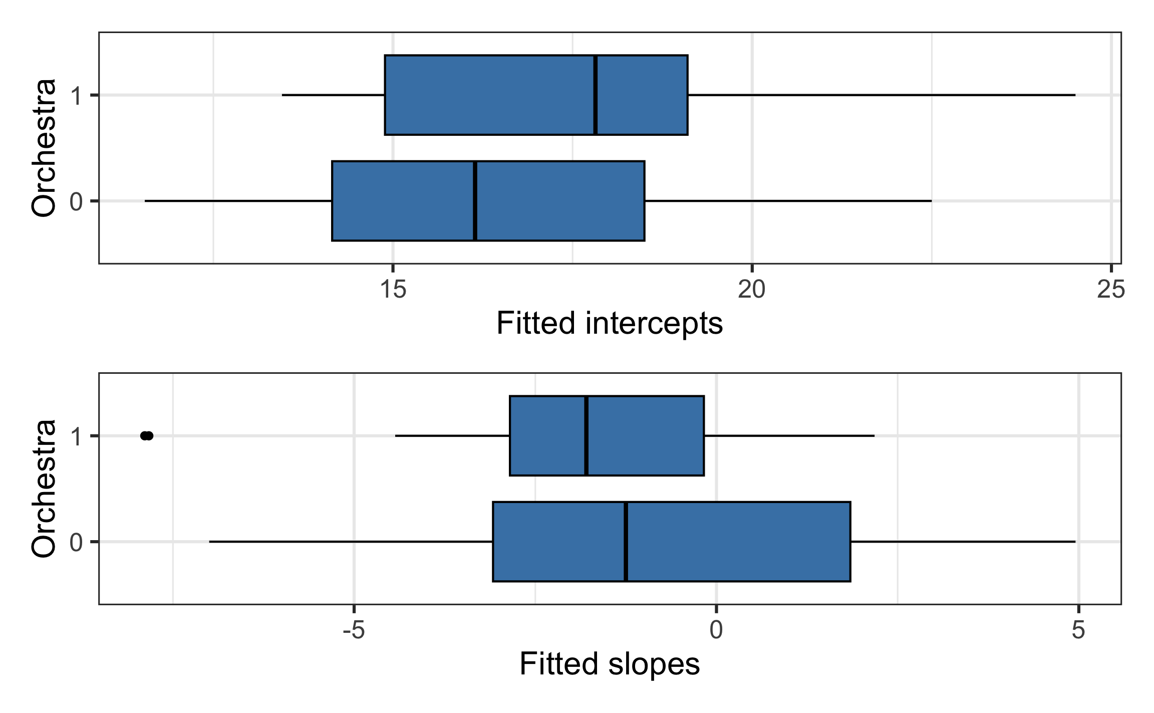
Level Two model
Model for intercepts
| term | estimate | std.error | statistic | p.value |
|---|---|---|---|---|
| (Intercept) | 16.283 | 0.671 | 24.249 | 0.000 |
| orchestra1 | 1.411 | 0.991 | 1.424 | 0.163 |
Model for slopes
| term | estimate | std.error | statistic | p.value |
|---|---|---|---|---|
| (Intercept) | -0.771 | 0.851 | -0.906 | 0.373 |
| orchestra1 | -1.406 | 1.203 | -1.168 | 0.253 |
Estimated two-level model
Level One
\[\hat{na}_{ij} = \hat{a}_i + \hat{b}_i ~ LargeEnsemble_{ij}\]
Level Two
\[\begin{aligned}&\hat{a}_i = 16.283 + 1.411 ~ Orchestra_i \\ &\hat{b}_i = -0.771 - 1.406 ~ Orchestra_i\end{aligned}\]
Estimated composite model
\[ \begin{aligned}\hat{na}_{ij} &= 16.283 + 1.411 ~ Orchestra_i - 0.771 ~ LargeEnsemble_{ij} \\ &- 1.406 ~ Orchestra_i:LargeEnsemble_{ij}\end{aligned} \]
(Note that we also have the error terms \(\epsilon_{ij}, u_i, v_i\) that we will discuss later)
Disadvantages to this approach
⚠️ Weighs each musician the same regardless of number of diary entries
⚠️ Drops subjects who have missing values for slope (7 individuals who didn’t play a large ensemble performance)
⚠️ Does not share strength effectively across individuals
We will use a unified approach that utilizes likelihood-based methods to address some of these drawbacks.
Unified approach to modeling multilevel data
Framework
Let \(Y_{ij}\) be the performance anxiety for the \(i^{th}\) musician before performance \(j\).
Level One
\[Y_{ij} = a_i + b_i ~ LargeEnsemble_{ij} + \epsilon_{ij}\]
Level Two
\[\begin{aligned}&a_i = \alpha_0 + \alpha_1 ~ Orchestra_i+ u_i\\ &b_i = \beta_0 + \beta_1~Orchestra_i + v_i\end{aligned}\]
Note
We will discuss the distribution of the error terms \(\epsilon_{ij}, u_i, v_i\) shortly.
Composite model
Plug in the equations for \(a_i\) and \(b_i\) to get the composite model \[\begin{aligned}Y_{ij} &= (\alpha_0 + \alpha_1 ~ Orchestra_i + \beta_0 ~ LargeEnsemble_{ij} \\ &+ \beta_1 ~ Orchestra_i:LargeEnsemble_{ij})\\ &+ (u_i + v_i ~ LargeEnsemble_{ij} + \epsilon_{ij})\end{aligned}\]
- The fixed effects to estimate are \(\alpha_0, \alpha_1, \beta_0, \beta_1\)
- The error terms are \(u_i, v_i, \epsilon_{ij}\)
- \(u_i\) and \(v_i\) are associated with musician random effect
- \(\epsilon_{ij}\) is what’s left unexplained
Note that we no longer need to estimate \(a_i\) and \(b_i\) directly as we did earlier. They conceptually connect the Level One and Level Two models.
Notation
Greek letters denote the fixed effect model parameters to be estimated
- e.g., \(\alpha_0, \alpha_1, \beta_0, \beta_1\)
Roman letters denote the preliminary fixed effects at lower levels (not directly estimated)
- e.g. \(a_i, b_i\)
\(\sigma\) and \(\rho\) denote variance components that will be estimated
\(\epsilon_{ij}, u_i, v_i\) denote error terms (not directly estimated)
Error terms
- We generally assume that the error terms are normally distributed, e.g. error associated with each performance of a given musician is \(\epsilon_{ij} \sim N(0, \sigma^2)\)
- For the Level Two models, the errors are
- \(u_i\): deviation of musician \(i\) from the mean performance anxiety before solos and small ensembles after accounting for the instrument
- musician-to-musician differences in the intercepts
- \(v_i\): deviance of musician \(i\) from the mean difference in performance anxiety between large ensembles and other performance types after accounting for instrument
- musician-to-musician differences in the slopes
- \(u_i\): deviation of musician \(i\) from the mean performance anxiety before solos and small ensembles after accounting for the instrument
- Need to account for fact that \(u_i\) and \(v_i\) are correlated for the \(i^{th}\) musician
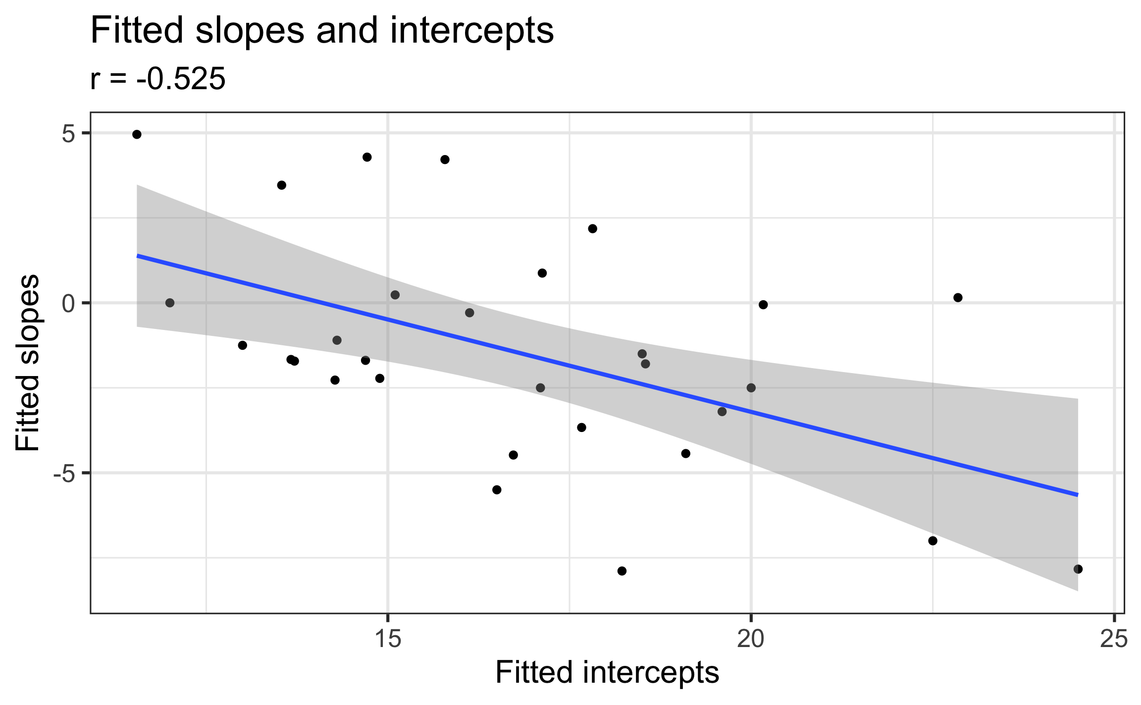
Recreated from Figure 8.11
Describe what we learn about the association between the slopes and intercepts based on this plot.
Distribution of Level Two errors
Use a multivariate normal distribution for the Level Two error terms \[\left[ \begin{array}{c} u_{i} \\ v_{i} \end{array} \right] \sim N \left( \left[ \begin{array}{c} 0 \\ 0 \end{array} \right], \left[ \begin{array}{cc} \sigma_{u}^{2} & \rho_{uv}\sigma_{u}\sigma_v \\ \rho_{uv}\sigma_{u}\sigma_v & \sigma_{v}^{2} \end{array} \right] \right)\]
where \(\sigma^2_u\) and \(\sigma^2_v\) are the variance of \(u_i\)’s and \(v_i\)’s respectively, and \(\sigma_{uv} = \rho_{uv}\sigma_u\sigma_v\) is covariance between \(u_i\) and \(v_i\)
- What does it mean for \(\rho_{uv} > 0\)?
- What does it mean for \(\rho_{uv} < 0\)?
Visualizing multivariate normal distribution
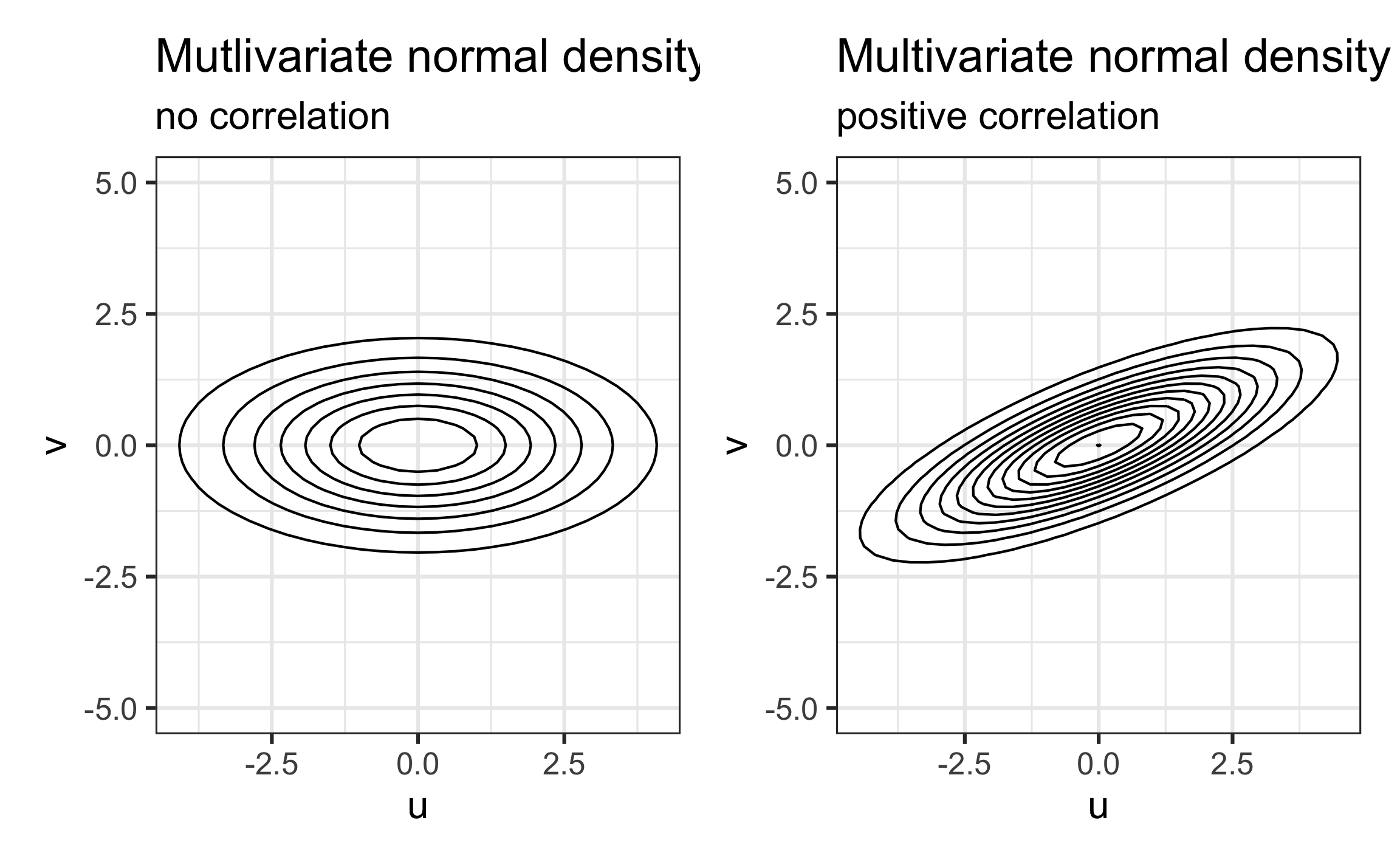
Recreated from Figure 8.12
Fit the model in R
Fit multilevel model using the lmer (“linear mixed effects in R”) function from the lme4 package.
na ~ orchestra + large_ensemble + orchestra:large_ensemble: Represents the fixed effects(large_ensemble|id): Represents the error terms and associated variance components- Specifies two error terms: \(u_i\) corresponding to the intercepts, \(v_i\) corresponding to effect of large ensemble
- Use
(1|id)for models with random intercepts and all other effects fixed.
Tidy output
Display results using the tidy function from the broom.mixed package.
Estimated fixed effects
Estimated random effects
| effect | group | term | estimate | std.error | statistic |
|---|---|---|---|---|---|
| ran_pars | id | sd__(Intercept) | 2.378 | NA | NA |
| ran_pars | id | cor__(Intercept).large_ensemble1 | -0.635 | NA | NA |
| ran_pars | id | sd__large_ensemble1 | 0.672 | NA | NA |
| ran_pars | Residual | sd__Observation | 4.670 | NA | NA |
Fitted model
\[ \begin{aligned} \hat{na}_{ij} &= 15.930 + 1.693 ~ Orchestra_i - 0.911 ~ LargeEnsemble_{ij} \\ &- 1.424 ~ Orchestra_i:LargeEnsemble_{ij} \\[30pt]&\left[ \begin{array}{c} u_{i} \\ v_{i} \end{array} \right] \sim N \left( \left[ \begin{array}{c} 0 \\ 0 \end{array} \right], \left[ \begin{array}{cc} 2.378^{2} & -0.635 *2.378 *0.672 \\ -0.635 *2.378 *0.672 & 0.672^{2} \end{array} \right] \right) \\[30pt] &\epsilon_{ij} \sim N(0, 4.670^2) \end{aligned} \]
Sadler and Miller (2010)
Read the Data Analysis Section in Sadler and Miller (2010). Click here to access the paper in Canvas. Use the text to answer the following:
- What is the goal of the analysis?
- What type of model is used? What is the response variable? What is the multilevel structure?
- Describe the details of the model estimation.
- Describe the data wrangling / creation of new variables. What were the goals of the data wrangling steps?
- How as model performance assessed?
06:00
Sadler and Miller 2010
Split into 3 - 5 groups and discuss your responses.
One person will write your group’s response to your assigned question(s).
Click here to access the slides.
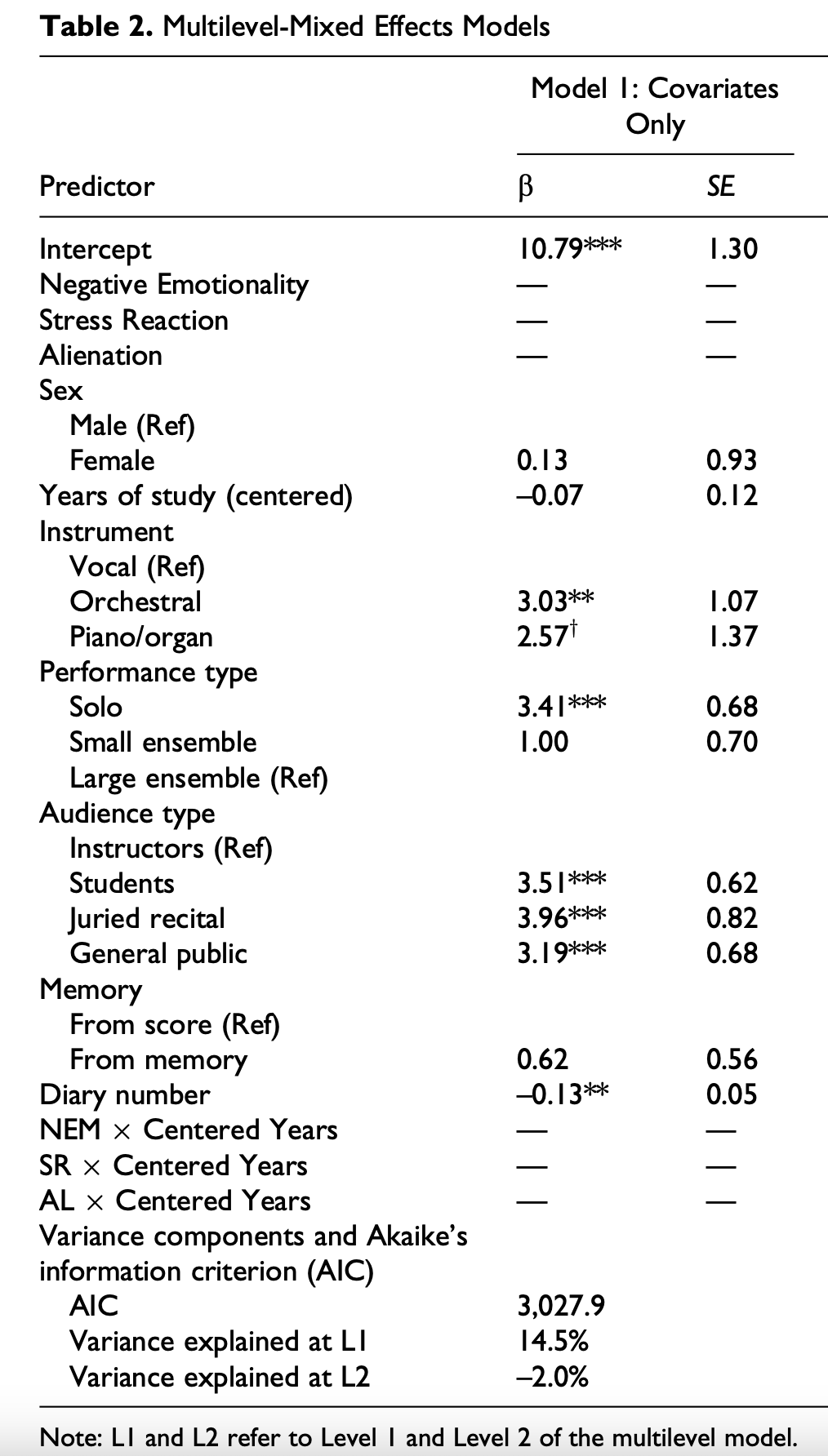
Sadler and Miller (2010) Model 1
