Correlated data
Feb 19, 2024
Announcements
Quiz 02: Tue, Feb 20, 9am - Thu, Feb 22, 12pm (noon)
Covers readings & lectures: Jan 24 - Feb 12
Poisson regression, unifying framework for GLMs, logistic regression, proportional odds models, probit regression
Read Sadler and Miller (2010) as part of Feb 26 prepare assignment
Learning goals
- Recognize a potential for correlation in a data set
- Identify observational units at varying levels
- Understand issues correlated data may cause in modeling
- Understand how random effects models can be used to take correlation into account
Correlated observations
Examples of correlated data
- In an education study, test scores for students from a particular teacher are typically more similar than test scores of other students with a different teacher
- In a study measuring depression indices weekly over a month, the four measures for the same patient tend to be more similar than depression indices from other patients
- In political polling, opinions of members from the same household tend to be more similar than opinions of members from another household
Correlation among outcomes within the same group (teacher, patient, household) is called intraclass correlation
Multilevel data
We can think of correlated data as a multilevel structure
Population elements are aggregated into groups
There are observational units and measurements at each level
For now we will focus on data with two levels:
- Level one: Most basic level of observation
- Level two: Groups formed from aggregated level-one observations
Multilevel data example
Example: education study
Level one
Observational units: students
Level-one covariates: test scores (response), year in school, demographics
Level two
Observational units: teachers
Level-two covariates:years of experience
Two types of effects in model
- Fixed effects: Effects that are of interest in the study
- Can think of these as effects whose interpretations would be included in a write up of the study
- Random effects: Not interested in studying effects of specific values in the data but we want to understand the variability
- Can think of these as effects whose interpretations would not necessarily be included in a write up of the study
Example
Researchers are interested in understanding the effect social media has on opinions about a proposed economic plan. They randomly select 1000 households. They ask each adult in the household how many minutes they spend on social media daily and whether they support the proposed economic plan.
- daily minutes on social media is the fixed effect
- household is the random effect
Practice
Radon is a carcinogen – a naturally occurring radioactive gas whose decay products are also radioactive – known to cause lung cancer in high concentrations. The EPA sampled more than 80,000 homes across the U.S. Each house came from a randomly selected county and measurements were made on each level of each home. Uranium measurements at the county level were included to improve the radon estimates.1
What are the level one and level two observational units?
What is the response variable and what is its type (normal, Poisson, etc.)?
Describe the within-group correlation.
What are the fixed effects? What are the random effects?
Teratogen and rat pups
Data: Teratogen and rat pups
Today’s data are simulated results of an experiment with 24 dams (mother rats) randomly divided into four groups that received different doses of teratogen, a substance that could potentially cause harm to developing fetuses. The four groups are
- High dose (3 mg)
- Medium dose (2 mg)
- Low dose (1 mg)
- No dose (Control)
Each dam produced 10 rat pups and the presence of a deformity was noted for each pup.
Goal: Understand the association between teratogen exposure and the probability a pup is born with a deformity.
Sources of variation
Dose effect: Studying whether different dose levels are associated with different probabilities of birth defects in the pups.
- Dose is a fixed effect. Study is interested in defect rate at specific dose levels.
Dam (litter) effect: Different dams may have different propensity to produce pups with defects, i.e. pups from same litter are more likely to be similar than pups from different litters.
- Dam is a random effect. Study is not interested in defect rate for each specific dam in the study but is interested in variability between litters.
Pup-to-pup variability: Within litter pup differences. This is the unexplained variability.
Scenario 1: No dose effect
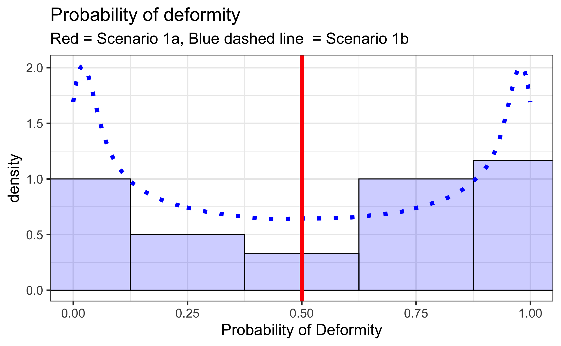
Assume dose has no effect on, \(p\), the probability of a pup born with a deformity.
Scenario 1a.: \(p = 0.5\) for each dam
Scenario 1b.: \(p \sim Beta(0.5, 0.5)\) (expected value = 0.5)
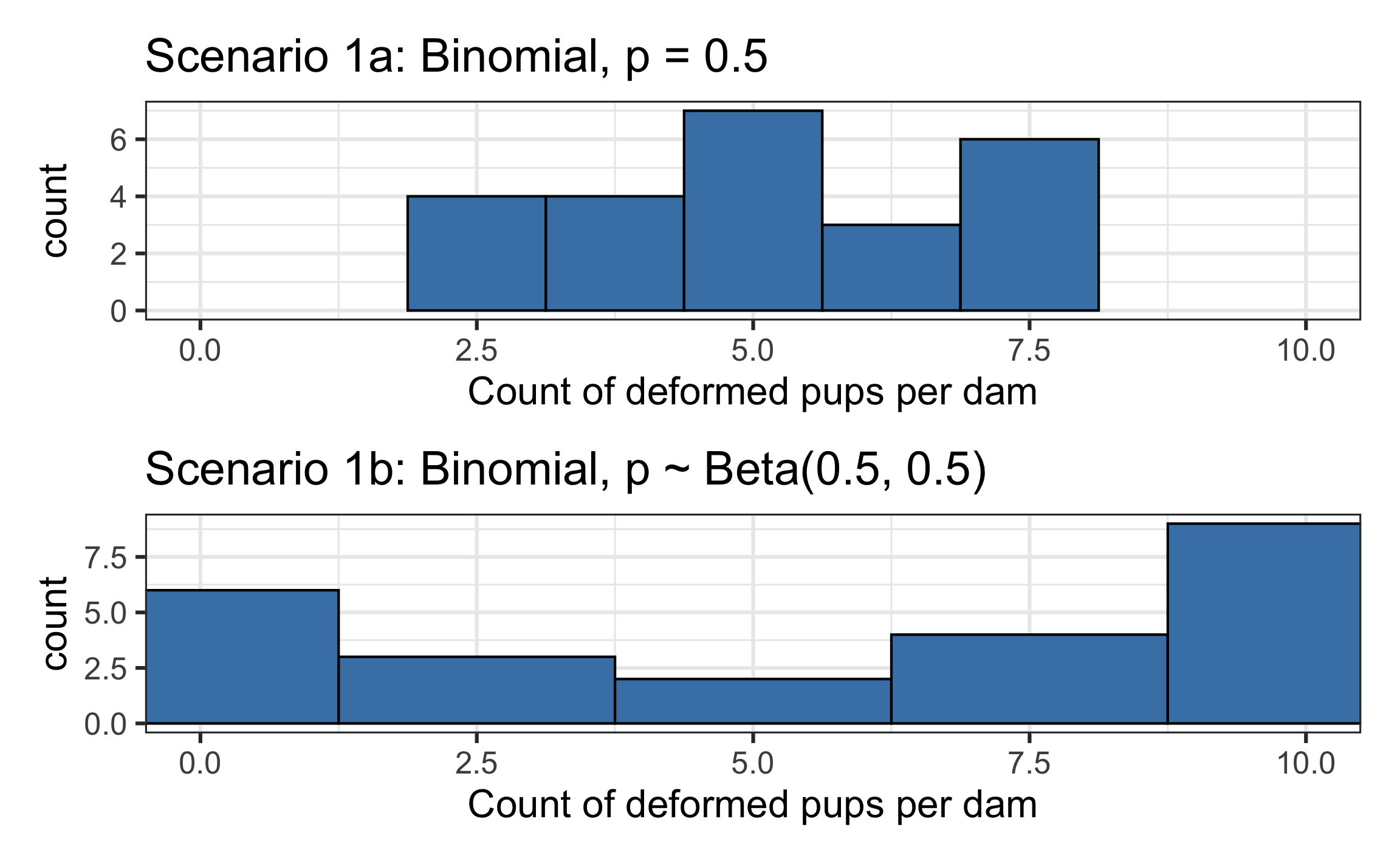
Would you expect the number of pups with a deformity for dams in Scenario 1a to follow a distribution similar to the binomial distribution with \(n=10\) and \(p=0.5\)? Why or why not?
Would you expect the number of pups with a deformity for dams in Scenario 1b to follow a distribution similar to the binomial distribution with \(n=10\) and \(p=0.5\)? Why or why not?
Which scenario do you think is more realistic - Scenario 1a or 1b?
| mean_1a | sd_1a | mean_1b | sd_1b |
|---|---|---|---|
| 5.166667 | 1.493949 | 5.666667 | 4.103727 |
Application exercise
Let’s take a look at a binomial and quasibinomial model for Scenarios 1a and 1b.
08:00
Scenario 2: Dose effect
Scenario 2: Dose effect
Now we will consider the effect of the dose of teratogen on the probability of a pup born with a deformity. The 24 pups have been randomly divided into four groups:
- High dose (
dose = 3) - Medium dose (
dose = 2) - Low dose (
dose = 1) - No dose (
dose = 0)
We will assume the true relationship between \(p\) and dose is the following:
\[\log\Big(\frac{p}{1-p}\Big) = -2 + 1.33 ~ dose\]
Scenario 2
Scenario 2a.
\[p = \frac{e^{-2 + 1.33 ~ dose}}{1 + e^{-2 + 1.33 ~ dose}}\]
Scenario 2b.
\[p \sim Beta\Big(\frac{2p}{(1-p)}, 2\Big)\]
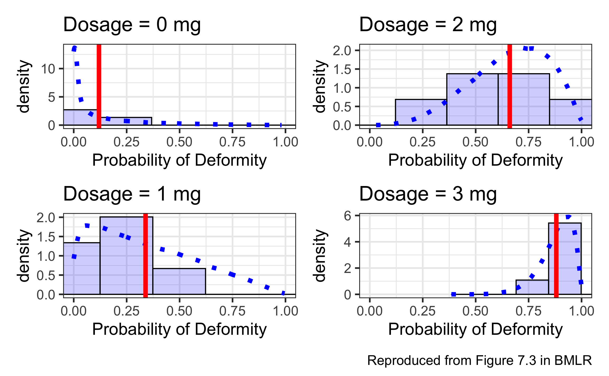
On average, dams who receive dose \(x\) have the same probability of pup born with deformity as dams with dose \(x\) under Scenario 2a.
- e.g., If
dose = 1, the probability of a pup born with deformity is 0.338 in Scenario 2a and the mean is 0.338 in Scenario 2b.
Distributions under Scenario 2
Scenario 2 summary statistics
Scenario 2a
|
Scenario 2b
|
|||||||
|---|---|---|---|---|---|---|---|---|
| Dosage | Mean p | SD p | Mean Count | SD Count | Mean p | SD p | Mean Count | SD Count |
| 0 | 0.119 | 0 | 1.333 | 1.366 | 0.061 | 0.069 | 0.500 | 0.837 |
| 1 | 0.339 | 0 | 3.167 | 1.835 | 0.239 | 0.208 | 3.500 | 2.881 |
| 2 | 0.661 | 0 | 5.833 | 1.472 | 0.615 | 0.195 | 5.833 | 1.941 |
| 3 | 0.881 | 0 | 8.833 | 1.169 | 0.872 | 0.079 | 8.833 | 1.169 |
- In Scenario 2a, dams produced 4.79 deformed pups on average, with standard deviation 3.20. Scenario 2b saw an average of 4.67 with standard deviation 3.58. Why are comparisons by dose more meaningful than these overall comparisons?
- We will use binomial and quasibinomial regression to model the relationship between dose and probability of pup born with a deformity. What can you say about the center and the width of the confidence intervals under Scenarios 2a and 2b?
- Which will be similar and why?
- Which will be different and how?
Scenario 2: Estimated odds ratio
The estimated effect of dose and the 95% CI from the binomial and quasibinomial models are below:
Scenario 2a
| Odds Ratio | 95% CI | |
|---|---|---|
| Binomial | 3.536 | (2.604, 4.958) |
| Quasibinomial | 3.536 | (2.512, 5.186) |
Scenario 2b
| Odds Ratio | 95% CI | |
|---|---|---|
| Binomial | 4.311 | (3.086, 6.271) |
| Quasibinomial | 4.311 | (2.735, 7.352) |
- Describe how the quasibinomial analysis of Scenario 2b differs from the binomial analysis of the same simulated data. Do confidence intervals contain the true model parameters? Is this what you expected? Why?
- Why does Scenario 2b contain correlated data that we must account for, while Scenario 2a does not?
Data structure
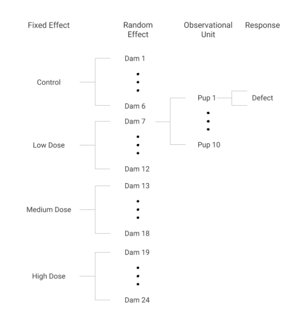
From Figure 7.4 in BMLR
Preview: Fit model with random effect
library(lme4)
library(broom.mixed)
random_effect_model <- glmer(deformity ~ dose + (1|dam),
                          family = binomial, data = scenario2_raw)
tidy(random_effect_model, conf.int = TRUE) |>
kable(digits = 3)| effect | group | term | estimate | std.error | statistic | p.value | conf.low | conf.high |
|---|---|---|---|---|---|---|---|---|
| fixed | NA | (Intercept) | -2.819 | 0.528 | -5.343 | 0 | -3.853 | -1.785 |
| fixed | NA | dose | 1.691 | 0.282 | 5.992 | 0 | 1.138 | 2.244 |
| ran_pars | dam | sd__(Intercept) | 0.834 | NA | NA | NA | NA | NA |
Summary
The structure of the data set may imply correlation between observations.
Correlated observations provide less information than independent observations; we need to account for this reduction in information.
Failing to account for this reduction could result in underestimating standard error, thus resulting in overstating significance and the precision of the estimates.
We showed how we can account for this by incorporating the dispersion parameter or a random effect.
