| age | sex | years | ppe_access |
|---|---|---|---|
| 34 | Male | 2 | 1 |
| 32 | Female | 3 | 1 |
| 32 | Female | 1 | 1 |
| 40 | Male | 4 | 1 |
| 32 | Male | 10 | 1 |
Logistic regression
Binomial responses + overdispersion
Feb 07, 2024
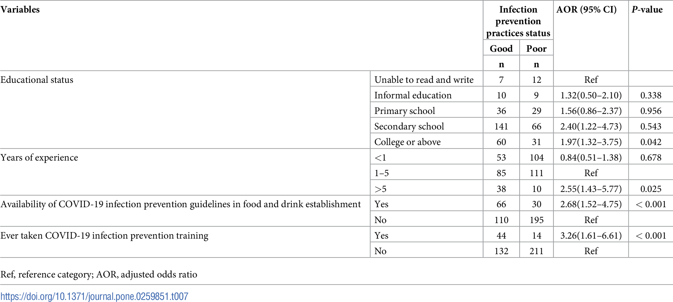
Results
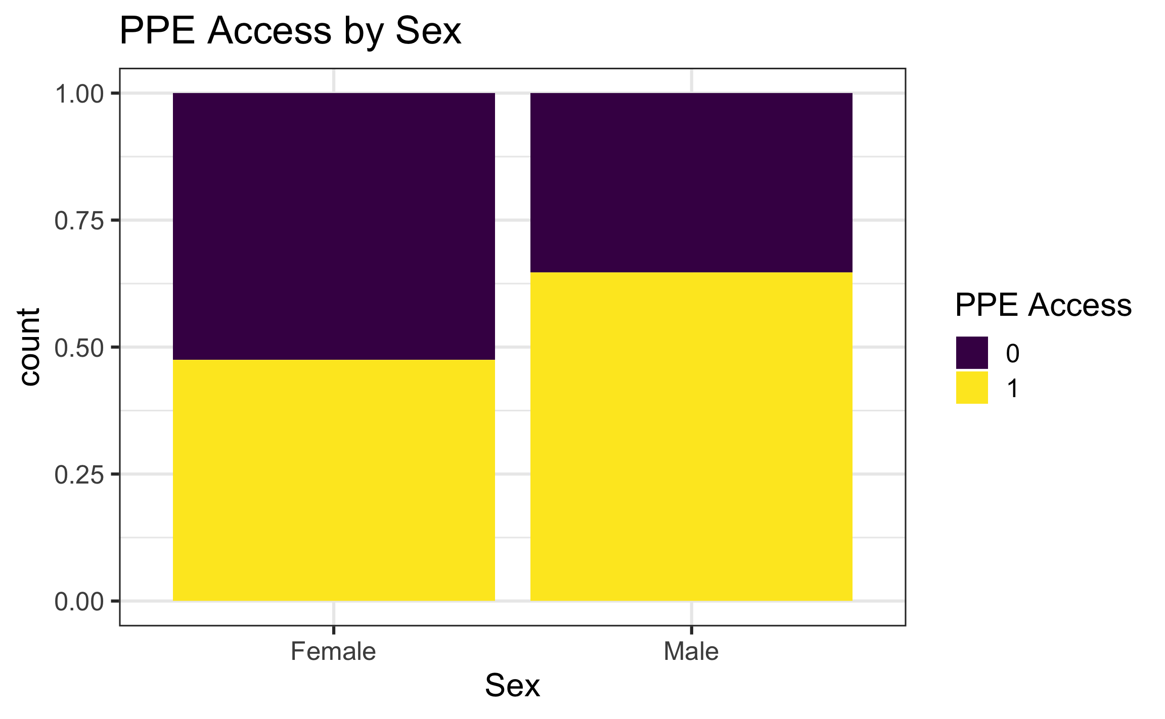
EDA for binary response
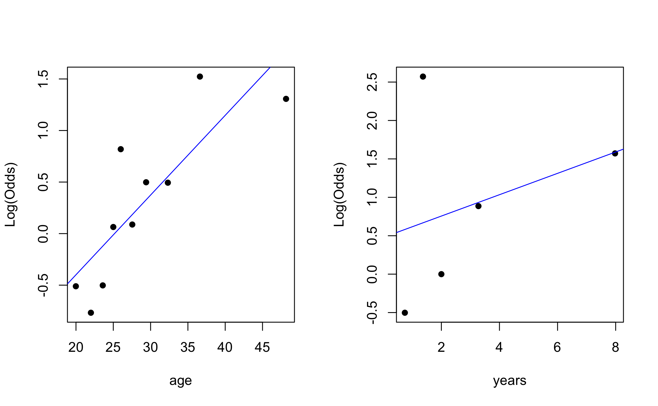
EDA for binary response
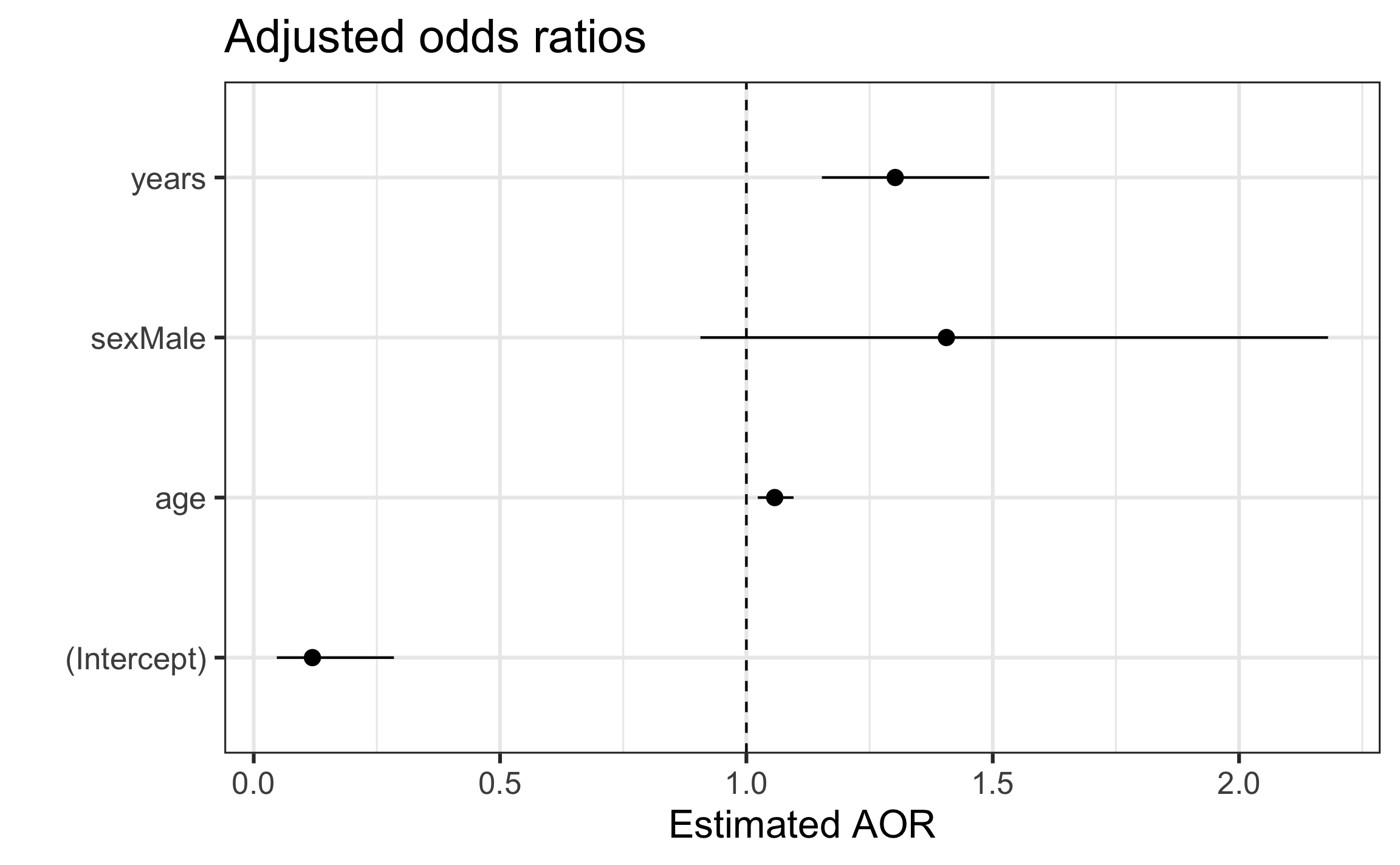
Visualizing coefficient estimates
Exploratory data analysis
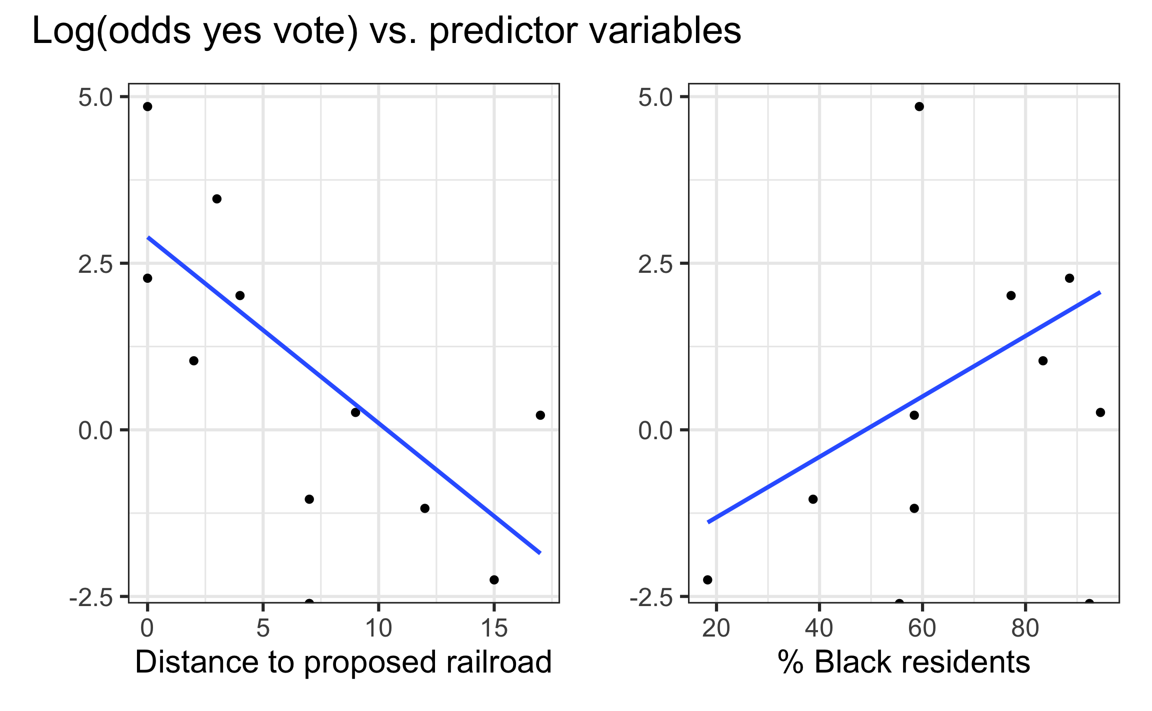
Exploratory data analysis
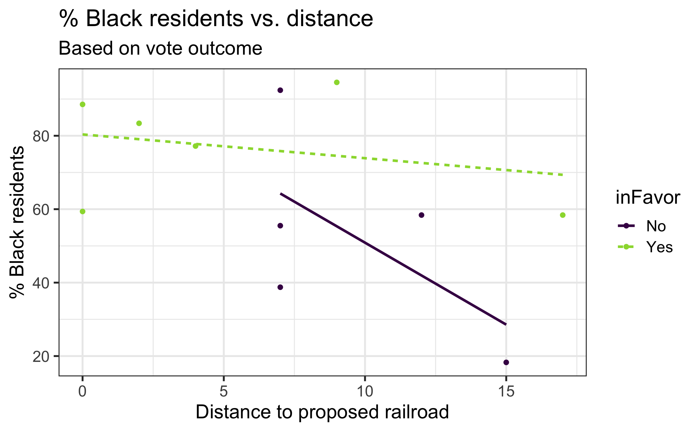
Check for potential multicollinearity and interaction effect.
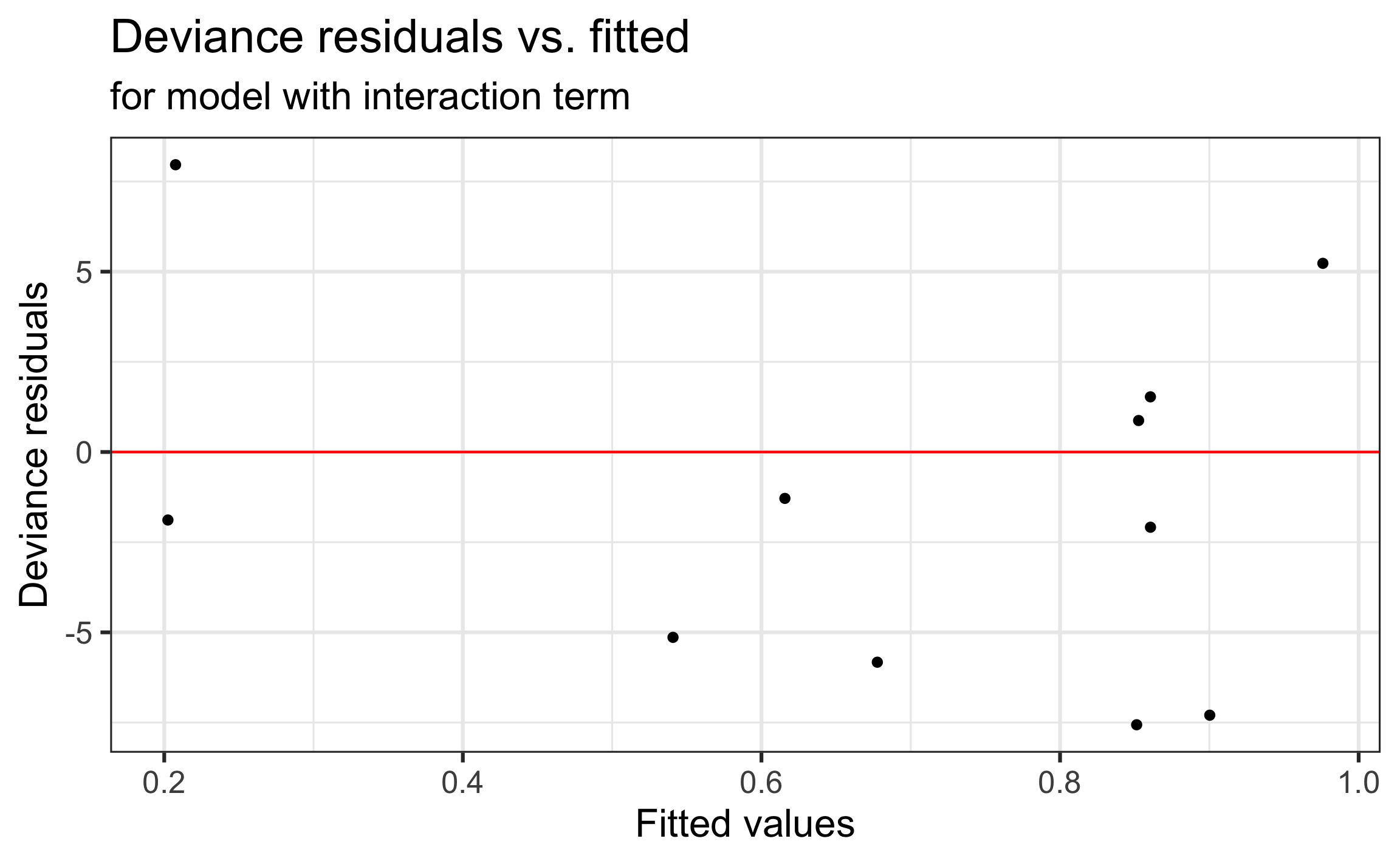
Plot of deviance residuals
References
![]()
Andualem, Atsedemariam, Belachew Tegegne, Sewunet Ademe, Tarikuwa Natnael, Gete Berihun, Masresha Abebe, Yeshiwork Alemnew, et al. 2022. “COVID-19 Infection Prevention Practices Among a Sample of Food Handlers of Food and Drink Establishments in Ethiopia.” PLoS One 17 (1): e0259851.
Roback, Paul, and Julie Legler. 2021. Beyond multiple linear regression: applied generalized linear models and multilevel models in R. CRC Press.