Poisson Regression
Jan 24, 2024
Computing set up
Topics
Describe properties of the Poisson random variable
Write the mathematical equation of the Poisson regression model
Describe how the Poisson regression differs from least-squares regression
Interpret the coefficients for the Poisson regression model
Compare two Poisson regression models
Scenarios to use Poisson regression
Does the number of employers conducting on-campus interviews during a year differ for public and private colleges?
Does the daily number of asthma-related visits to an Emergency Room differ depending on air pollution indices?
Does the number of paint defects per square foot of wall differ based on the years of experience of the painter?
Each response variable is a count per a unit of time or space.
Poisson distribution
Let \(Y\) be the number of events in a given unit of time or space. Then \(Y\) can be modeled using a Poisson distribution
\[P(Y=y) = \frac{e^{-\lambda}\lambda^y}{y!} \hspace{10mm} y=0,1,2,\ldots, \infty\]
Features
- \(E(Y) = Var(Y) = \lambda\)
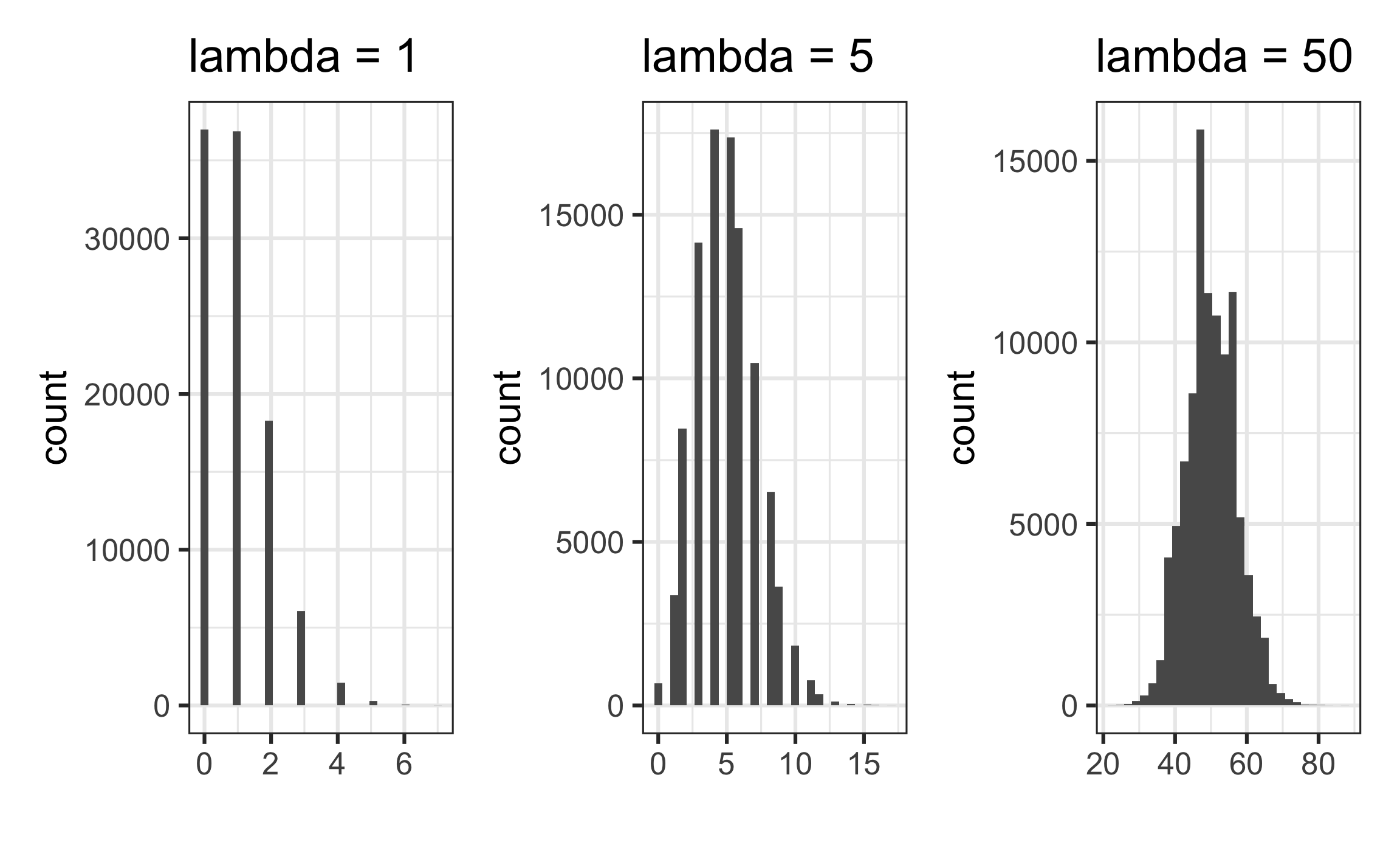
- The distribution is typically skewed right, particularly if \(\lambda\) is small
- The distribution becomes more symmetric as \(\lambda\) increases
- If \(\lambda\) is sufficiently large, it can be approximated using a normal distribution (Click here for an example.)
| Mean | Variance | |
|---|---|---|
| lambda = 1 | 0.99351 | 0.9902178 |
| lambda = 5 | 4.99367 | 4.9865798 |
| lambda = 50 | 49.99288 | 49.8962683 |
Example1
The annual number of earthquakes registering at least 2.5 on the Richter Scale and having an epicenter within 40 miles of downtown Memphis follows a Poisson distribution with mean 6.5. What is the probability there will be at 3 or fewer such earthquakes next year?
\[P(Y \leq 3) = P(Y = 0) + P(Y = 1) + P(Y = 2) + P(Y = 3)\]
\[ = \frac{e^{-6.5}6.5^0}{0!} + \frac{e^{-6.5}6.5^1}{1!} + \frac{e^{-6.5}6.5^2}{2!} + \frac{e^{-6.5}6.5^3}{3!}\]
\[ = 0.112\]
Poisson regression
The data: Household size in the Philippines
The data fHH1.csv come from the 2015 Family Income and Expenditure Survey conducted by the Philippine Statistics Authority.
Goal: Understand the association between household size and various characteristics of the household
Response:
total: Number of people in the household other than the head
Predictors:
location: Where the house is locatedage: Age of the head of householdroof: Type of roof on the residence (proxy for wealth)
Other variables:
numLT5: Number in the household under 5 years old
The data
| location | age | total | numLT5 | roof |
|---|---|---|---|---|
| CentralLuzon | 65 | 0 | 0 | Predominantly Strong Material |
| MetroManila | 75 | 3 | 0 | Predominantly Strong Material |
| DavaoRegion | 54 | 4 | 0 | Predominantly Strong Material |
| Visayas | 49 | 3 | 0 | Predominantly Strong Material |
| MetroManila | 74 | 3 | 0 | Predominantly Strong Material |
Response variable
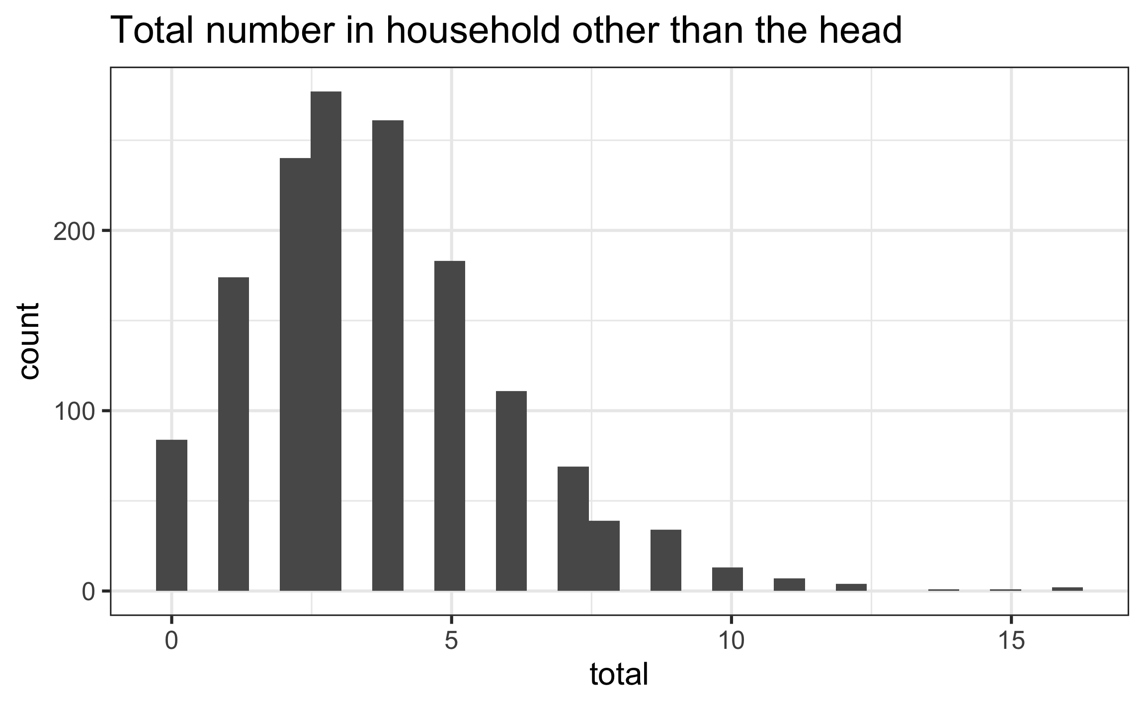
| mean | var |
|---|---|
| 3.685 | 5.534 |
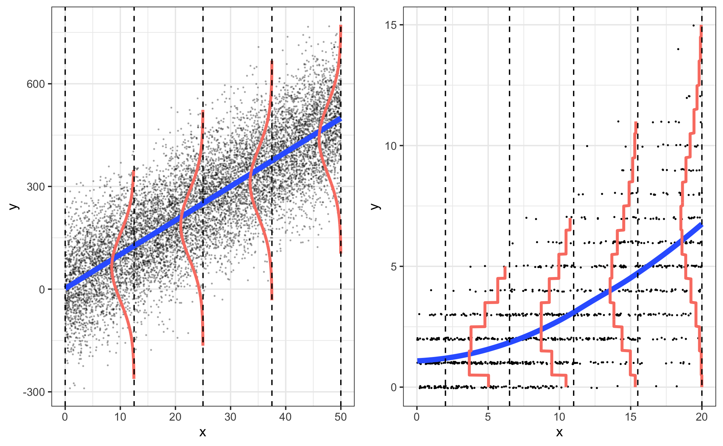
Why the least-squares model doesn’t work
The goal is to model \(\lambda\), the expected number of people in the household (other than the head), as a function of the predictors (covariates)
We might be tempted to try a linear model \[\lambda_i = \beta_0 + \beta_1x_{i1} + \beta_2x_{i2} + \dots + \beta_px_{ip}\]
This model won’t work because…
- It could produce negative values of \(\lambda\) for certain values of the predictors
- The equal variance assumption required to conduct inference for linear regression is violated.
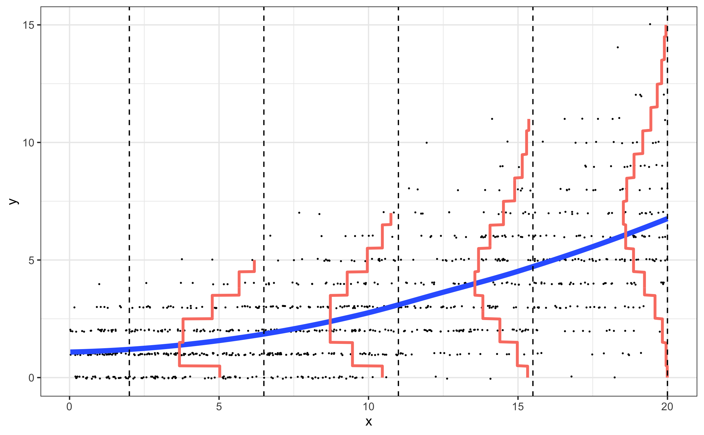
Poisson regression model
If \(Y_i \sim Poisson\) with \(\lambda = \lambda_i\) for the given values \(x_{i1}, \ldots, x_{ip}\), then
\[\log(\lambda_i) = \beta_0 + \beta_1 x_{i1} + \beta_2 x_{i2} + \dots + \beta_p x_{ip}\]
Each observation can have a different value of \(\lambda\) based on its value of the predictors \(x_1, \ldots, x_p\)
\(\lambda\) determines the mean and variance, so we don’t need to estimate a separate error term
Poisson vs. multiple linear regression
Assumptions for Poisson regression
Poisson response: The response variable is a count per unit of time or space, described by a Poisson distribution, at each level of the predictor(s)
Independence: The observations must be independent of one another
Mean = Variance: The mean must equal the variance
Linearity: The log of the mean rate, \(\log(\lambda)\), must be a linear function of the predictor(s)
Model 1: Household vs. Age
| term | estimate | std.error | statistic | p.value |
|---|---|---|---|---|
| (Intercept) | 1.5499 | 0.0503 | 30.8290 | 0 |
| age | -0.0047 | 0.0009 | -5.0258 | 0 |
\[\log(\hat{\lambda}) = 1.5499 - 0.0047 ~ age\]
The coefficient for age is -0.0047. Interpret this coefficient in context. Select all that apply.
The mean household size is predicted to decrease by 0.0047 for each year older the head of the household is.
The mean household size is predicted to multiply by a factor of 0.9953 for each year older the head of the household is.
The mean household size is predicted to decrease by 0.9953 for each year older the head of the household is.
The mean household size is predicted to multiply by a factor of 0.47% for each year older the head of the household is.
The mean household size is predicted to decrease by 0.47% for each year older the head of the household is.
Is the coefficient of age statistically significant?
| term | estimate | std.error | statistic | p.value | conf.low | conf.high |
|---|---|---|---|---|---|---|
| (Intercept) | 1.5499 | 0.0503 | 30.8290 | 0 | 1.4512 | 1.6482 |
| age | -0.0047 | 0.0009 | -5.0258 | 0 | -0.0065 | -0.0029 |
\[H_0: \beta_1 = 0 \hspace{2mm} \text{ vs. } \hspace{2mm} H_a: \beta_1 \neq 0\]
Test statistic
\[Z = \frac{\hat{\beta}_1 - 0}{SE(\hat{\beta}_1)} = \frac{-0.0047 - 0}{0.0009} = -5.026 \text{ (using exact values)}\]
P-value
\[P(|Z| > |-5.026|) = 5.01 \times 10^{-7} \approx 0\]
What are plausible values for the coefficient of age?
| term | estimate | std.error | statistic | p.value | conf.low | conf.high |
|---|---|---|---|---|---|---|
| (Intercept) | 1.5499 | 0.0503 | 30.8290 | 0 | 1.4512 | 1.6482 |
| age | -0.0047 | 0.0009 | -5.0258 | 0 | -0.0065 | -0.0029 |
95% confidence interval for the coefficient of age
\[\hat{\beta}_1 \pm z^{*}\times SE(\hat{\beta}_1)\]
where \(z^* \sim N(0, 1)\) \[-0.0047 \pm 1.96 \times 0.0009 = \mathbf{(-.0065, -0.0029)}\]
Interpret the interval in terms of the change in mean household size.
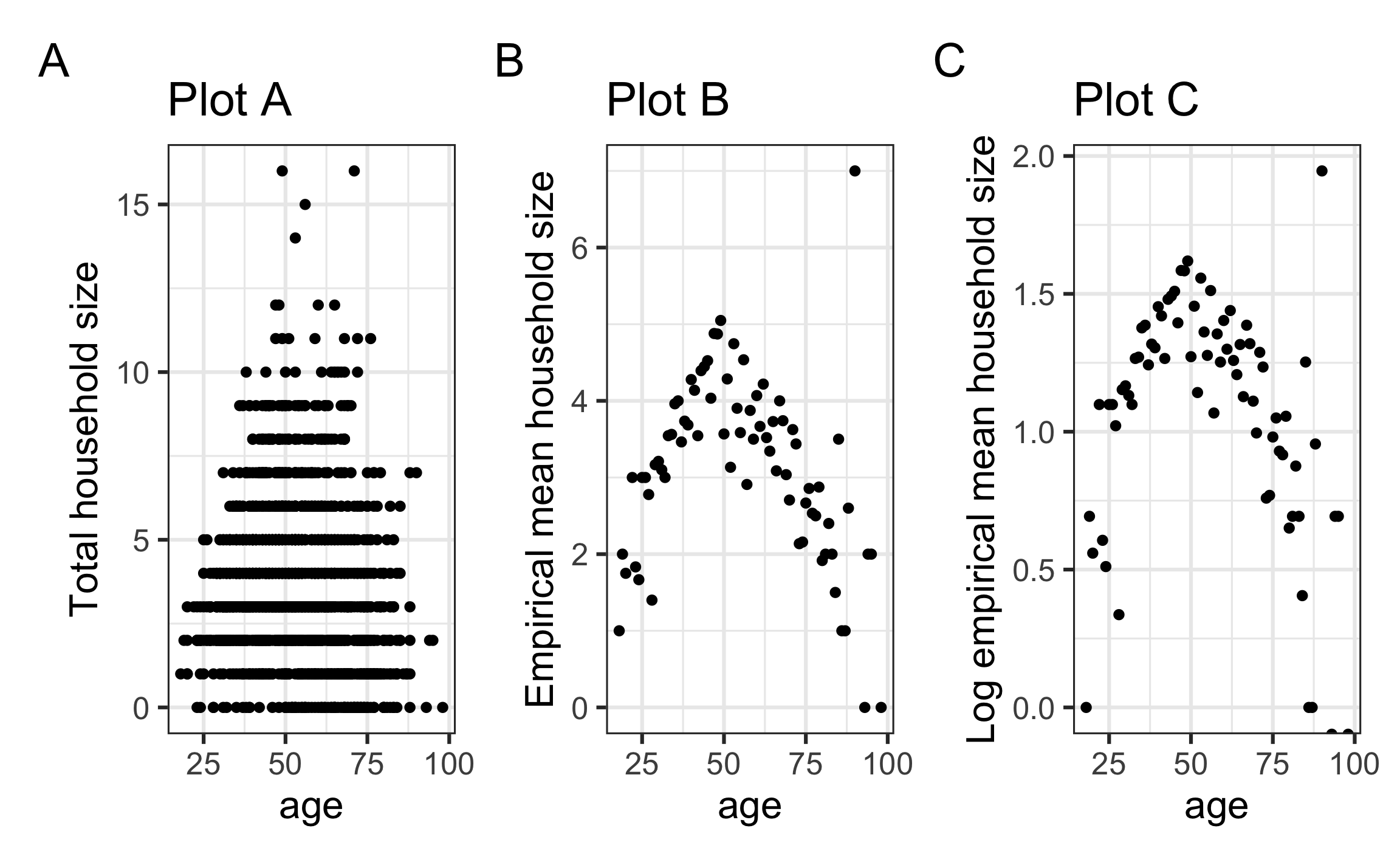
Which plot can best help us determine whether Model 1 is a good fit?
Model 2: Add a quadratic effect for age
hh_data <- hh_data |>
  mutate(age2 = age*age)

model2 <- glm(total ~ age + age2, data = hh_data, family = poisson)
tidy(model2, conf.int = T) |>
kable(digits = 4)| term | estimate | std.error | statistic | p.value | conf.low | conf.high |
|---|---|---|---|---|---|---|
| (Intercept) | -0.3325 | 0.1788 | -1.8594 | 0.063 | -0.6863 | 0.0148 |
| age | 0.0709 | 0.0069 | 10.2877 | 0.000 | 0.0575 | 0.0845 |
| age2 | -0.0007 | 0.0001 | -11.0578 | 0.000 | -0.0008 | -0.0006 |
Model 2: Add a quadratic effect for age
| term | estimate | std.error | statistic | p.value | conf.low | conf.high |
|---|---|---|---|---|---|---|
| (Intercept) | -0.3325 | 0.1788 | -1.8594 | 0.063 | -0.6863 | 0.0148 |
| age | 0.0709 | 0.0069 | 10.2877 | 0.000 | 0.0575 | 0.0845 |
| age2 | -0.0007 | 0.0001 | -11.0578 | 0.000 | -0.0008 | -0.0006 |
We can determine whether to keep \(age^2\) in the model in two ways:
1️⃣ Use the p-value (or confidence interval) for the coefficient (since we are adding a single term to the model)
2️⃣ Conduct a drop-in-deviance test
Deviance
A deviance is a way to measure how the observed data differs (deviates) from the model predictions.
It’s a measure unexplained variability in the response variable (similar to SSE in linear regression )
Lower deviance means the model is a better fit to the data
We can calculate the “deviance residual” for each observation in the data (more on the formula later). Let \((\text{deviance residual}_i\) be the deviance residual for the \(i^{th}\) observation, then
\[\text{deviance} = \sum(\text{deviance residual})_i^2\]
Note: Deviance is also known as the “residual deviance”
Drop-in-Deviance Test
We can use a drop-in-deviance test to compare two models. To conduct the test
1️⃣ Compute the deviance for each model
2️⃣ Calculate the drop in deviance
\[\text{drop-in-deviance = Deviance(reduced model) - Deviance(larger model)}\]
3️⃣ Given the reduced model is the true model \((H_0 \text{ true})\), then \[\text{drop-in-deviance} \sim \chi_d^2\]
where \(d\) is the difference in degrees of freedom between the two models (i.e., the difference in number of terms)
Drop-in-deviance to compare Model1 and Model2
| Resid. Df | Resid. Dev | Df | Deviance | Pr(>Chi) |
|---|---|---|---|---|
| 1498 | 2337.089 | NA | NA | NA |
| 1497 | 2200.944 | 1 | 136.145 | 0 |
- Write the null and alternative hypotheses.
- What does the value 2337.089 tell you?
- What does the value 1 tell you?
- What is your conclusion?
Add location to the model?
Suppose we want to add location to the model, so we compare the following models:
Model A: \(\lambda_i = \beta_0 + \beta_1 ~ age_i + \beta_2 ~ age_i^2\)
Model B: \(\lambda_i = \beta_0 + \beta_1 ~ age_i + \beta_2 ~ age_i^2 + \beta_3 ~ Loc1_i + \beta_4 ~ Loc2_i + \beta_5 ~ Loc3_i + \beta_6 ~ Loc4_i\)
Which of the following are reliable ways to determine if location should be added to the model?
- Drop-in-deviance test
- Use the p-value for each coefficient
- Likelihood ratio test
- Nested F Test
- BIC
Looking ahead
- For next time - Chapter 4 - Poisson Regression
- Sections 4.6, 4.10