Review of multiple linear regression

Part 2

class: middle, center

##Click for PDF of slides

---

Announcements

• Lab starts Thu 3:30 - 4:45pm online
  • Find Zoom link in Sakai
• Office hours this week:
  • Thu 2 - 3pm & Fri 1 - 2pm online (links in Sakai)
  • Full office hours schedule starts Tue, Jan 19
• Week 02 reading: BMLR: Chapter 2- Beyond Least Squares: Using Likelihoods

---

class: middle

Questions?

---

class: middle, inverse

Recap

---

Data: Kentucky Derby Winners

.midi[ Today’s data is from the Kentucky Derby, an annual 1.25-mile horse race held at the Churchill Downs race track in Louisville, KY. The data is in the file derbyplus.csv and contains information for races 1896 - 2017. ]

.pull-left[

.midi[Response variable]

• .midi[speed: Average speed of the winner in feet per second (ft/s)]

.midi[Additional variable] .midi[- winner: Winning horse] ]

.pull-right[ .midi[Predictor variables] - .midi[year: Year of the race] - .midi[condition: Condition of the track (good, fast, slow)] - .midi[starters: Number of horses who raced]]

---

Data

derby <- read_csv("data/derbyplus.csv") %>%
  mutate(yearnew = year - 1896)

derby %>%
  head(5) %>% kable()

year	winner	condition	speed	starters	yearnew
1896	Ben Brush	good	51.66	8	0
1897	Typhoon II	slow	49.81	6	1
1898	Plaudit	good	51.16	4	2
1899	Manuel	fast	50.00	5	3
1900	Lieut. Gibson	fast	52.28	7	4

---

Model 1: Main effects model (with centering)

term	estimate	std.error	statistic	p.value
(Intercept)	52.175	0.194	269.079	0.000
starters	-0.005	0.017	-0.299	0.766
yearnew	0.023	0.002	9.766	0.000
conditiongood	-0.443	0.231	-1.921	0.057
conditionslow	-1.543	0.161	-9.616	0.000

---

Model 2: Include quadratic effect for year

.midi[

term	estimate	std.error	statistic	p.value
(Intercept)	51.4130	0.1826	281.5645	0.0000
starters	-0.0253	0.0136	-1.8588	0.0656
yearnew	0.0700	0.0061	11.4239	0.0000
I(yearnew^2)	-0.0004	0.0000	-8.0411	0.0000
conditiongood	-0.4770	0.1857	-2.5689	0.0115
conditionslow	-1.3927	0.1305	-10.6701	0.0000

]

---

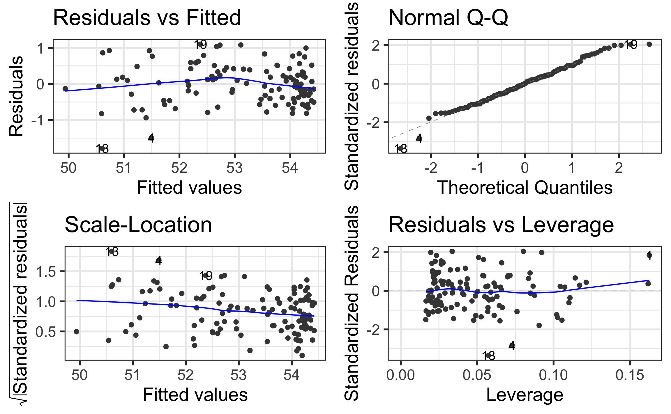
Model 2: Check model assumptions

---

class: middle, inverse

## Model 3

Include interaction term?

Recall from the EDA…

---

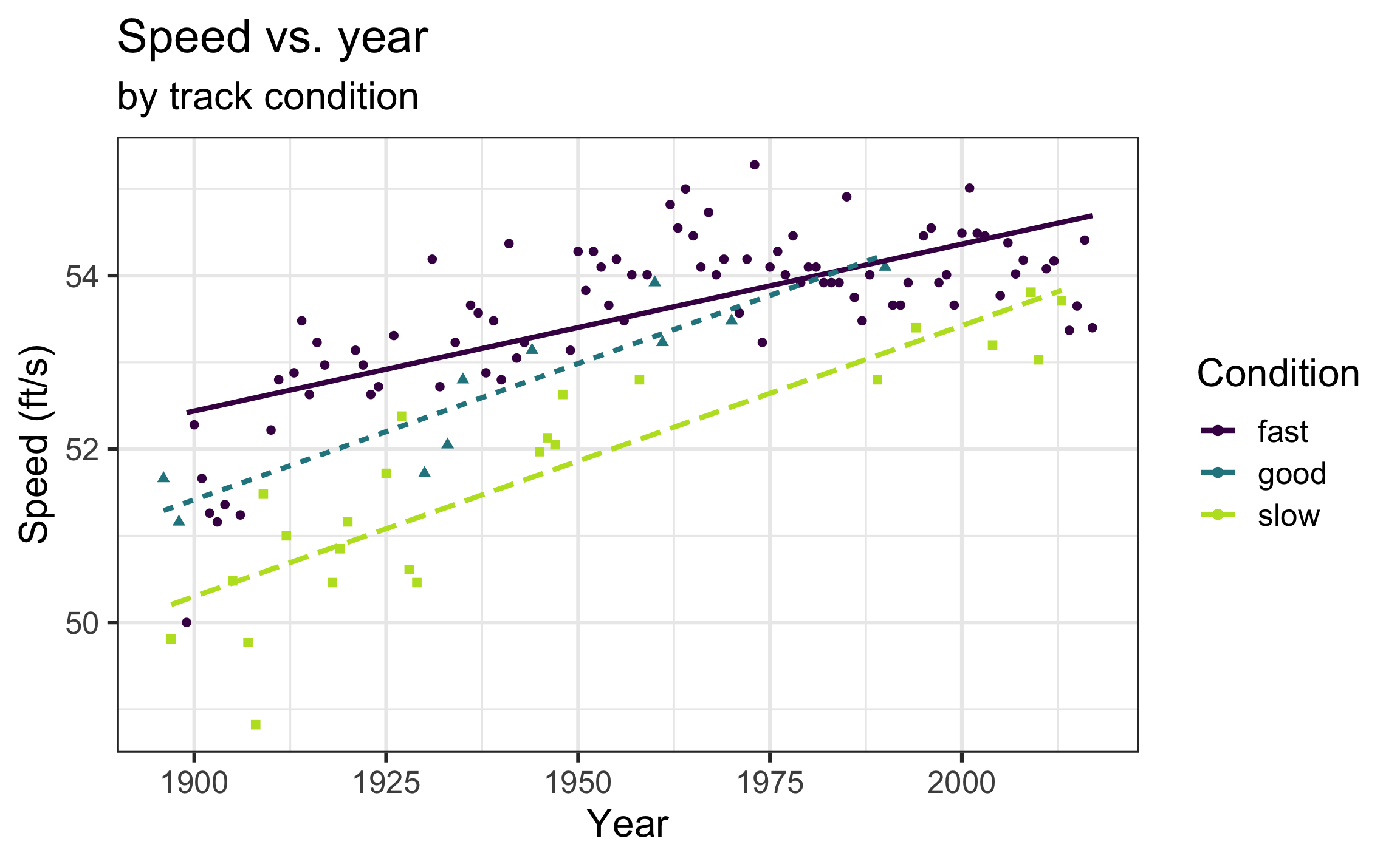
Model 3: Include interaction term

$$\begin{array}{rl}\widehat{speed}=& 52.387-0.003starters+0.020yearnew-1.070good-2.183slow\\ & +0.012yearnew\times good+0.012yearnew\times slow\end{array}$$

.panelset.sideways[ .panel[.panel-name[Output]

term	estimate	std.error	statistic	p.value
(Intercept)	52.387	0.200	262.350	0.000
starters	-0.003	0.016	-0.189	0.850
yearnew	0.020	0.003	7.576	0.000
conditiongood	-1.070	0.423	-2.527	0.013
conditionslow	-2.183	0.270	-8.097	0.000
yearnew:conditiongood	0.012	0.008	1.598	0.113
yearnew:conditionslow	0.012	0.004	2.866	0.005

]

.panel[.panel-name[Code]

model3 <- lm(speed ~ starters + yearnew + condition +
               yearnew * condition, 
             data = derby)
tidy(model3) %>% kable(digits = 4)

] .panel[.panel-name[Assumptions]

] ]

---

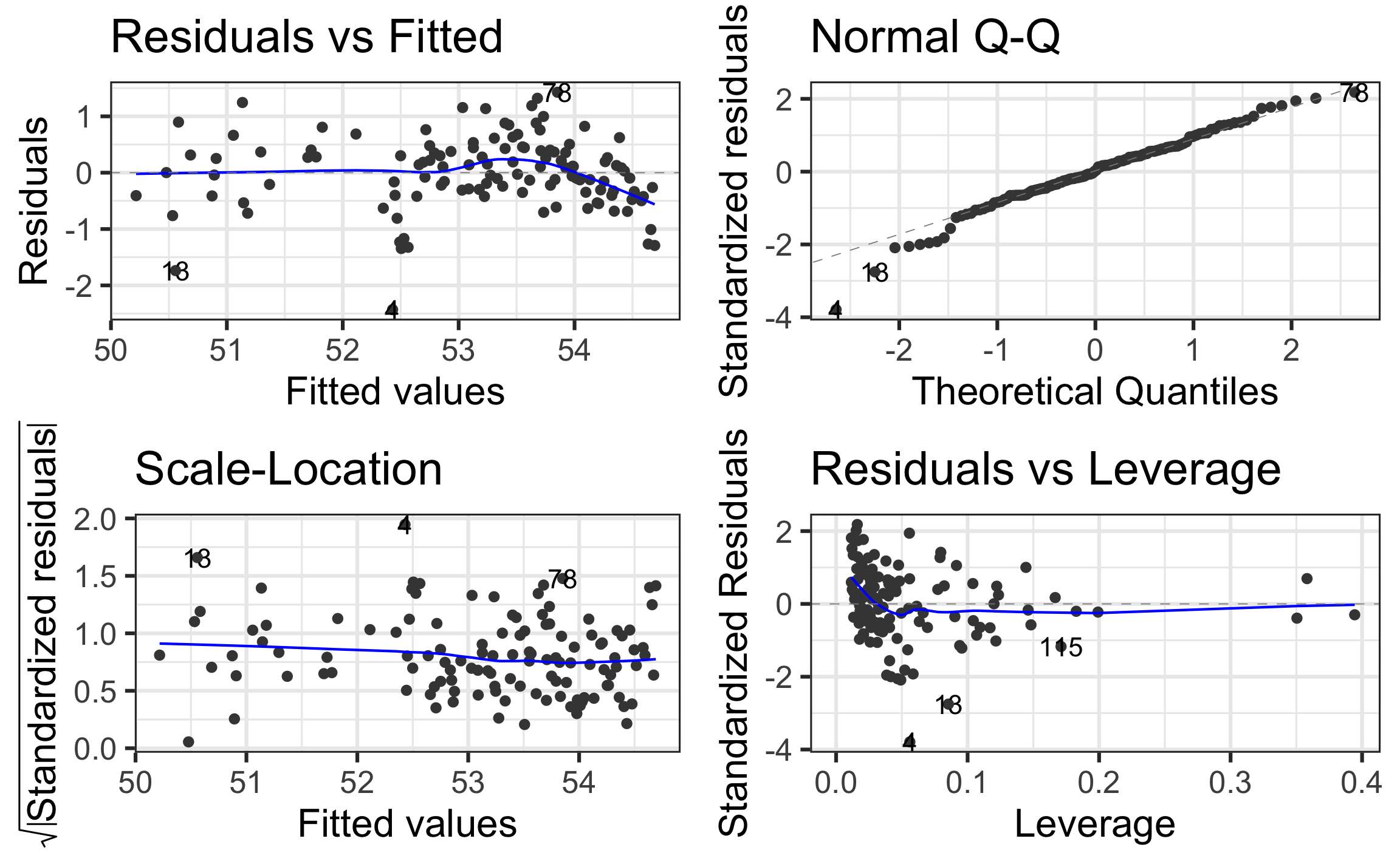
Interpreting interaction effects

term	estimate	std.error	statistic	p.value
(Intercept)	52.387	0.200	262.350	0.000
starters	-0.003	0.016	-0.189	0.850
yearnew	0.020	0.003	7.576	0.000
conditiongood	-1.070	0.423	-2.527	0.013
conditionslow	-2.183	0.270	-8.097	0.000
yearnew:conditiongood	0.012	0.008	1.598	0.113
yearnew:conditionslow	0.012	0.004	2.866	0.005

Click here for poll

04:00

---

Measures of model performance

• $R^2$: Proportion of variability in the response explained by the model.
  • Will always increase as predictors are added, so it shouldn’t be used to compare models
• $Adj.R^2$: Similar to $R^2$ with a penalty for extra terms

–

• $AIC$: Likelihood-based approach balancing model performance and complexity

• $BIC$: Similar to AIC with stronger penalty for extra terms

–

• Nested F Test (extra sum of squares F test): Generalization of t-test for individual coefficients to perform significance tests on nested models

---

Which model would you choose?

Use the glance function to get model statistics.

model	r.squared	adj.r.squared	AIC	BIC
Model1	0.730	0.721	259.478	276.302
Model2	0.827	0.819	207.429	227.057
Model3	0.751	0.738	253.584	276.016

Which model would you choose?

Characteristics of a “good” final model

• Model can be used to answer primary research questions
• Predictor variables control for important covariates
• Potential interactions have been investigated
• Variables are centered, as needed, for more meaningful interpretations
• Unnecessary terms are removed
• Assumptions are met and influential points have been addressed
• Model tells a “persuasive story parsimoniously”

.footnote[List from Section 1.6.7 of BMLR]

---

class: middle, inverse

Inference for multiple linear regression

---

Inference for regression

Use statistical inference to

• Determine if predictors are statistically significant (not necessarily practically significant!)
• Quantify uncertainty in coefficient estimates
• Quantify uncertainty in model predictions

If L.I.N.E. assumptions are met, we can conduct inference using the $t$ distribution and estimated standard errors

---

Inference for regression

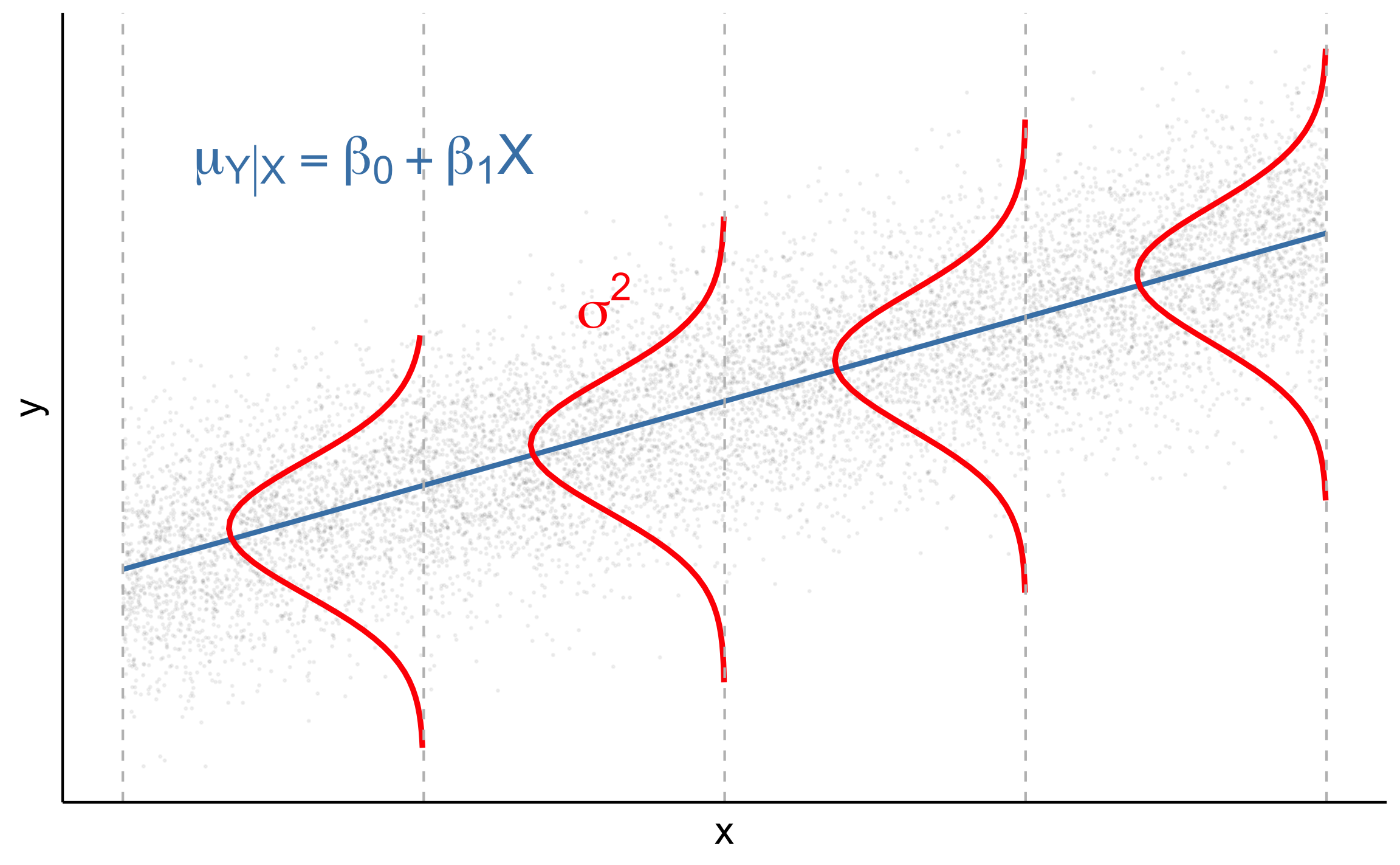
.pull-left[

When L.I.N.E. conditions are met

]

.pull-right[

• Use least squares regression to get the estimates ${\hat{\beta }}_0$, ${\hat{\beta }}_1$, and ${\hat{\sigma }}^2$

• $\hat{\sigma }$ is the regression standard error

$$\hat{\sigma }=\sqrt{\frac{\sum _{i=1}^n(y_i-{\hat{y}}_i{)}^2}{n-p-1}}=\sqrt{\frac{\sum _{i=1}^n{e}_i^2}{n-p-1}}$$

where $p$ is the number of non-intercept terms in the model

(p = 1 in simple linear regression) ]

---

Inference for ${\beta }_j$

• Suppose we have the following model:

$$y_i={\beta }_0+{\beta }_1{x}_{1i}+{\beta }_2{x}_{2i}+\cdots +{\beta }_p{x}_{pi}+{ϵ}_iϵ\sim N(0,{\sigma }^2)$$

–

• We use least squares regression to get estimates for the parameters ${\beta }_0,{\beta }_1,\dots ,{\beta }_p$ and ${\sigma }^2$. The regression equation is

$$\hat{y}={\hat{\beta }}_0+{\hat{\beta }}_1{x}_1+{\hat{\beta }}_2{x}_2+\cdots +{\hat{\beta }}_p{x}_p$$

• When the L.I.N.E. assumptions are met, ${\hat{\beta }}_j\sim N({\beta }_j,S{E}_{{\hat{\beta }}_j})$.
  • The objective of statistical inference is to understand ${\beta }_j$
  • Use $\hat{\sigma }$ to estimate $S{E}_{{\hat{\beta }}_j}$, the standard error of ${\hat{\beta }}_j$

---

Inference for ${\beta }_j$

.eq[ $$S{E}_{{\hat{\beta }}_j}=\hat{\sigma }\sqrt{\frac{1}{(n-1)s_{x_j}^2}}$$]

Conduct inference for ${\beta }_j$ using a $t$ distribution with $n-p-1$ degrees of freedom (df).

• ${\hat{\beta }}_j$ follows a $t$ distribution, because $\hat{\sigma }$ (not $\sigma$) is used to calculate the standard error of ${\hat{\beta }}_j$.

• The distribution has $n-p-1$ df because we use up $p+1$ df to calculate $\hat{\sigma }$, so there are $n-p-1$ df left to understand variability.

---

Hypothesis test for ${\beta }_j$

.pull-left[ 1️⃣ State the hypotheses

.eq[ $$H_0:{\beta }_j=0\text{ vs. }{H}_a:{\beta }_j\ne 0$$]

2️⃣ Calculate the test statistic.

.eq[ $$t=\frac{{\hat{\beta }}_j-0}{S{E}_{{\hat{\beta }}_j}}=\frac{{\hat{\beta }}_j-0}{\hat{\sigma }\sqrt{\frac{1}{(n-1)s_{x_j}^2}}}$$] ]

.pull-right[ 3️⃣ Calculate the p-value.

.eq[ $$\text{p-value}=2P(T>|t|)T\sim t_{n-p-1}$$]

4️⃣ State the conclusion in context of the data.

.eq[ Reject $H_0$ if p-value is sufficiently small.]

]

---

Confidence intervals

.eq[ The $C$% confidence confidence interval for ${\beta }_j$ is

$$\begin{array}{rl}& {\hat{\beta }}_j\pm t^{\ast }\times S{E}_{{\hat{\beta }}_j}\\ & {\hat{\beta }}_j\pm t^{\ast }\times \hat{\sigma }\sqrt{\frac{1}{(n-1)s_{x_j}^2}}\end{array}$$ where the critical value $t^{\ast }\sim t(n-p-1)$ ]

General interpretation: We are $C$% confident that for every one unit increase in $x_j$, the response is expected to change by LB to UB units, holding all else constant.

---

Inference Activity (~8 minutes)

• Use the Model 3 output on the next slide to conduct a hypothesis test and interpret the 95% confidence interval for your assigned variable.

  • You do not have to do the calculations by hand.

• Choose one person to write your group’s response on your slide slide.

• Choose on person to share your group’s responses with the class.

---

Model 3 output

term	estimate	std.error	statistic	p.value	conf.low	conf.high
(Intercept)	52.387	0.200	262.350	0.000	51.991	52.782
starters	-0.003	0.016	-0.189	0.850	-0.035	0.029
yearnew	0.020	0.003	7.576	0.000	0.014	0.025
conditiongood	-1.070	0.423	-2.527	0.013	-1.908	-0.231
conditionslow	-2.183	0.270	-8.097	0.000	-2.717	-1.649
yearnew:conditiongood	0.012	0.008	1.598	0.113	-0.003	0.027
yearnew:conditionslow	0.012	0.004	2.866	0.005	0.004	0.020

---

Additional review topics

• Uncertainty in predictions

• Variable transformations

• Comparing models using Nested F tests

---

Acknowledgements

These slides are based on content in BMLR: Chapter 1 - Review of Multiple Linear Regression