Using likelihoods

Prof. Maria Tackett

Jan 22, 2024

Announcements

• HW 01 due Wednesday at 11:59pm

Computing set up

library(tidyverse)
library(tidymodels)
library(GGally)
library(knitr)
library(patchwork)
library(viridis)
library(ggfortify)

ggplot2::theme_set(ggplot2::theme_bw(base_size = 16))
colors <- tibble::tibble(green = "#B5BA72")

Topics

• Review inference for multiple linear regression

• Using likelihoods

Notes based on Chapter 1 and 2 of Roback and Legler (2021) unless noted otherwise.

Inference for multiple linear regression

Data: Kentucky Derby Winners

Today’s data is from the Kentucky Derby, an annual 1.25-mile horse race held at the Churchill Downs race track in Louisville, KY. The data is in the file derbyplus.csv and contains information for races 1896 - 2017.

Response variable

• speed: Average speed of the winner in feet per second (ft/s)

Additional variable

• winner: Winning horse

Predictor variables

• year: Year of the race
• condition: Condition of the track (good, fast, slow)
• starters: Number of horses who raced

Goal: Understand variability in average winner speed based on characteristics of the race.

Data

derby <- read_csv("data/derbyplus.csv")

derby |>
  head(5) |> kable()

year	winner	condition	speed	starters
1896	Ben Brush	good	51.66	8
1897	Typhoon II	slow	49.81	6
1898	Plaudit	good	51.16	4
1899	Manuel	fast	50.00	5
1900	Lieut. Gibson	fast	52.28	7

Candidate models

Model 1: Main effects model (year, condition, starters)

model1 <- lm(speed ~ starters + year + condition, data = derby)

Model 2: Main effects + \(year^2\), the quadratic effect of year

model2 <- lm(speed ~ starters + year + I(year^2) + condition,
             data = derby)

Model 3: Main effects + interaction between year and condition

model3 <- lm(speed ~ starters + year + condition + year * condition, 
             data = derby)

Inference for regression

Use statistical inference to

• Evaluate if predictors are statistically significant (not necessarily practically significant!)

• Quantify uncertainty in coefficient estimates

• Quantify uncertainty in model predictions

If LINE assumptions are met, we can use inferential methods based on mathematical models. If at least linearity and independence are met, we can use simulation-based inference methods.

Inference for regression

When LINE assumptions are met… . . .

• Use least squares regression to obtain the estimates for the model coefficients \(\beta_0, \beta_1, \ldots, \beta_j\) and for \(\sigma^2\)

• \(\hat{\sigma}\) is the regression standard error

  \[ \hat{\sigma} = \sqrt{\frac{\sum_{i=1}^n(y_i - \hat{y}_i)^2}{n - p - 1}} = \sqrt{\frac{\sum_{i=1}^n e_i^2}{n-p-1}} \]

  where \(p\) is the number of non-intercept terms in the model (e.g., \(p = 1\) in simple linear regression)

• Goal is to use estimated values to draw conclusions about \(\beta_j\)

  • Use \(\hat{\sigma}\) to calculate \(SE_{\hat{\beta}_j}\) . Click here for more detail.

Hypothesis testing for \(\beta_j\)

1. State the hypotheses. \(H_0: \beta_j = 0 \text{ vs. } H_a: \beta_j \neq 0\), given the other variables in the model.

2. Calculate the test statistic.

\[ t = \frac{\hat{\beta}_j - 0}{SE_{\hat{\beta}_j}} \]

3. Calculate the p-value. The p-value is calculated from a \(t\) distribution with \(n - p - 1\) degrees of freedom.

   \[ \text{p-value} = 2P(T > |t|) \hspace{4mm} T \sim t_{n-p-1} \]

4. State the conclusion in context of the data.
   • Reject \(H_0\) if p-value is sufficiently small.

Confidence interval for \(\beta_j\)

The \(C\%\) confidence confidence interval for \(\beta_j\) is

\[\hat{\beta}_j \pm t^* \times SE_{\hat{\beta}_j}\]

where the critical value \(t^* \sim t_{n-p-1}\)

General interpretation for the confidence interval [LB, UB]:

We are \(C\%\) confident that for every one unit increase in \(x_j\), the response is expected to change by LB to UB units, holding all else constant.

Application exercise

📋 sta310-sp24.netlify.app/ae/ae-02-mlr-review

Measures of model performance

• \(R^2\): Proportion of variability in the response explained by the model

  • Will always increase as predictors are added, so it shouldn’t be used to compare models

• \(Adj. R^2\): Similar to \(R^2\) with a penalty for extra terms

• \(AIC\): Likelihood-based approach balancing model performance and complexity

• \(BIC\): Similar to AIC with stronger penalty for extra terms

Model summary statistics

Use the glance() function to get model summary statistics

model	r.squared	adj.r.squared	AIC	BIC
Model1	0.730	0.721	259.478	276.302
Model2	0.827	0.819	207.429	227.057
Model3	0.751	0.738	253.584	276.016

Which model do you choose based on these statistics?

Characteristics of a “good” final model

• Model can be used to answer primary research questions

• Predictor variables control for important covariates

• Potential interactions have been investigated

• Variables are centered, as needed, for more meaningful interpretations

• Unnecessary terms are removed

• Assumptions are met and influential points have been addressed

• Model tells a “persuasive story parsimoniously”

List from Section 1.6.7 of Roback and Legler (2021)

Using likelihoods

Learning goals

• Describe the concept of a likelihood

• Construct the likelihood for a simple model

• Define the Maximum Likelihood Estimate (MLE) and use it to answer an analysis question

• Identify three ways to calculate or approximate the MLE and apply these methods to find the MLE for a simple model

• Use likelihoods to compare models

What is the likelihood?

A likelihood is a function that tells us how likely we are to observe our data for a given parameter value (or values).

• Unlike Ordinary Least Squares (OLS), they do not require the responses be independent, identically distributed, and normal (iidN)

• They are not the same as probability functions

Probability function vs. likelihood

• Probability function: Fixed parameter value(s) + input possible outcomes \(\Rightarrow\) probability of seeing the different outcomes given the parameter value(s)

• Likelihood: Fixed data + input possible parameter values \(\Rightarrow\) probability of seeing the fixed data for each parameter value

Data: Fouls in college basketball games

The data set 04-refs.csv includes 30 randomly selected NCAA men’s basketball games played in the 2009 - 2010 season.¹

We will focus on the variables foul1, foul2, and foul3, which indicate which team had a foul called them for the 1st, 2nd, and 3rd fouls, respectively.

• H: Foul was called on the home team
• V: Foul was called on the visiting team

We are focusing on the first three fouls for this analysis, but this could easily be extended to include all fouls in a game.

1. The dataset was derived from basektball0910.csv used in BMLR Section 11.2

Fouls in college basketball games

refs <- read_csv("data/04-refs.csv")
refs |> slice(1:5) |> kable()

game	date	visitor	hometeam	foul1	foul2	foul3
166	20100126	CLEM	BC	V	V	V
224	20100224	DEPAUL	CIN	H	H	V
317	20100109	MARQET	NOVA	H	H	H
214	20100228	MARQET	SETON	V	V	H
278	20100128	SETON	SFL	H	V	V

We will treat the games as independent in this analysis.

Different likelihood models

Model 1 (Unconditional Model):

• What is the probability the referees call a foul on the home team, assuming foul calls within a game are independent?

Model 2 (Conditional Model):

• Is there a tendency for the referees to call more fouls on the visiting team or home team?

• Is there a tendency for referees to call a foul on the team that already has more fouls?

Ultimately we want to decide which model is better.

Exploratory data analysis

refs |>
count(foul1, foul2, foul3) |> kable()

foul1	foul2	foul3	n
H	H	H	3
H	H	V	2
H	V	H	3
H	V	V	7
V	H	H	7
V	H	V	1
V	V	H	5
V	V	V	2

There are

• 46 total fouls on the home team
• 44 total fouls on the visiting team

Model 1: Unconditional model

What is the probability the referees call a foul on the home team, assuming foul calls within a game are independent?

Likelihood

Let \(p_H\) be the probability the referees call a foul on the home team. The likelihood for a single observation \[Lik(p_H) = p_H^{y_i}(1 - p_H)^{n_i - y_i}\]Where \(y_i\) is the number of fouls called on the home team. (In this example, we know \(n_i = 3\) for all observations.)

Example

For a single game where the first three fouls are \(H, H, V\), then \[Lik(p_H) = p_H^{2}(1 - p_H)^{3 - 2} = p_H^{2}(1 - p_H)\]

Model 1: Likelihood contribution

Foul 1	Foul 2	Foul 3	n	Likelihood contribution
H	H	H	3	\(p_H^3\)
H	H	V	2	\(p_H^2(1 - p_H)\)
H	V	H	3	\(p_H^2(1 - p_H)\)
H	V	V	7	A
V	H	H	7	B
V	H	V	1	\(p_H(1 - p_H)^2\)
V	V	H	5	\(p_H(1 - p_H)^2\)
V	V	V	2	\((1 - p_H)^3\)

Fill in A and B.

02:00

Model 1: Likelihood function

Because the observations (the games) are independent, the likelihood is

\[Lik(p_H) = \prod_{i=1}^{n}p_H^{y_i}(1 - p_H)^{3 - y_i}\]

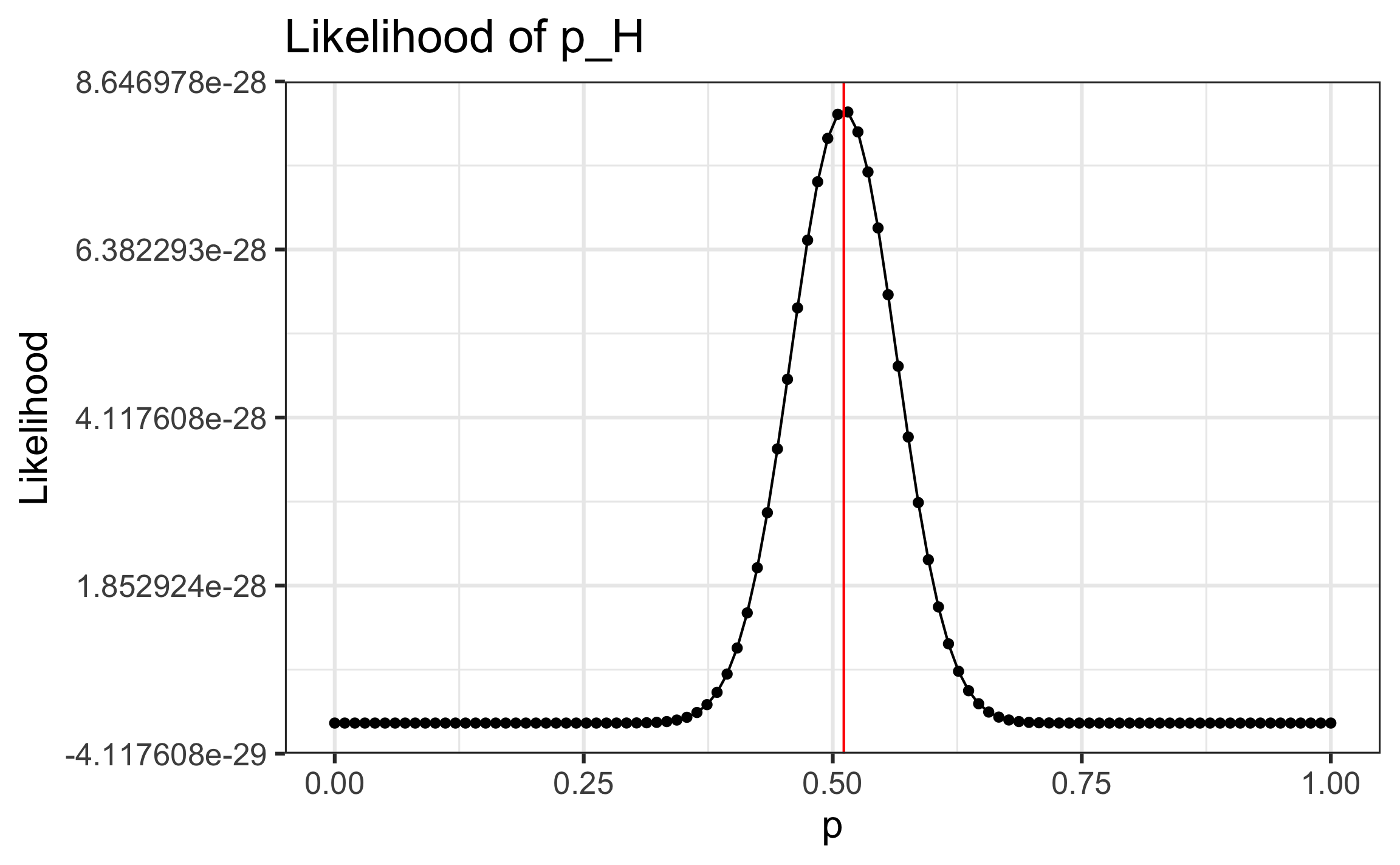
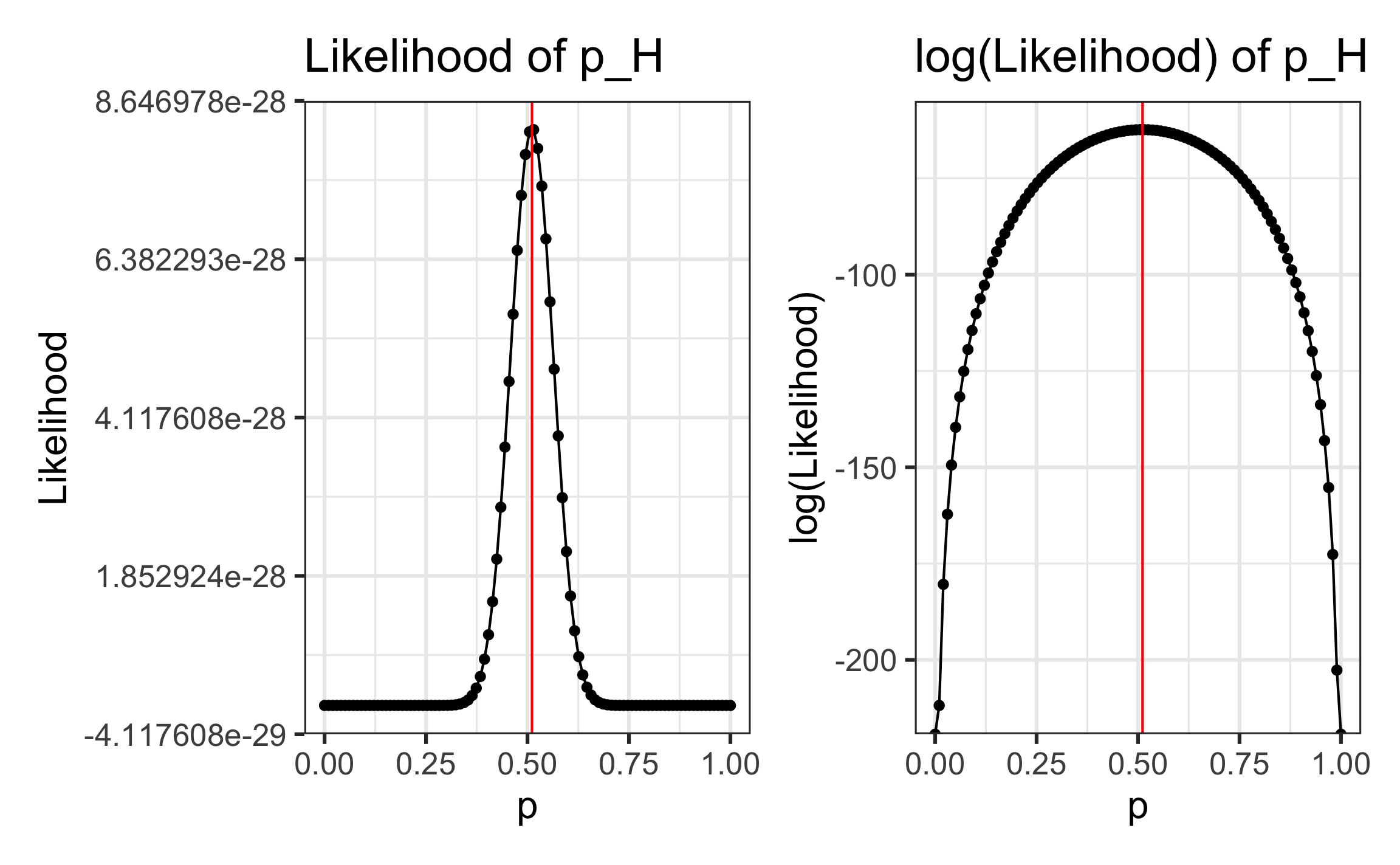
We will use this function to find the maximum likelihood estimate (MLE). The MLE is the value between 0 and 1 where we are most likely to see the observed data.

Visualizing the likelihood

What is your best guess for the MLE, $\hat{p}_H$?

1. 0.489
2. 0.500
3. 0.511
4. 0.556

Finding the maximum likelihood estimate

There are three primary ways to find the MLE

✅ Approximate using a graph

✅ Numerical approximation

✅ Using calculus

Approximate MLE from a graph

Find the MLE using numerical approximation

Specify a finite set of possible values the for \(p_H\) and calculate the likelihood for each value

# write an R function for the likelihood
ref_lik <- function(ph) {
  ph^46 *(1 - ph)^44
}

# search possible values for p and return max
nGrid = 1000
ph <- seq(0, 1, length = nGrid)
lik <- ref_lik(ph)
ph[lik == max(lik)]

[1] 0.5115115

# use the optimize function to find the MLE
optimize(ref_lik, interval = c(0,1), maximum = TRUE)

$maximum
[1] 0.5111132

$objective
[1] 8.25947e-28

Find MLE using calculus

• Find the MLE by taking the first derivative of the likelihood function.

• This can be tricky because of the Product Rule, so we can maximize the log(Likelihood) instead. The same value maximizes the likelihood and log(Likelihood)

Find MLE using calculus

\[Lik(p_H) = \prod_{i=1}^{n}p_H^{y_i}(1 - p_H)^{3 - y_i}\]

\[ \begin{aligned}\log(Lik(p_H)) &= \sum_{i=1}^{n}y_i\log(p_H) + (3 - y_i)\log(1 - p_H)\\[10pt] &= 46\log(p_H) + 44\log(1 - p_H)\end{aligned} \]

Find MLE using calculus

\[\frac{d}{d p_H} \log(Lik(p_H)) = \frac{46}{p_H} - \frac{44}{1-p_H} = 0\]

\[\Rightarrow \frac{46}{p_H} = \frac{44}{1-p_H}\]

\[\Rightarrow 46(1-p_H) = 44p_H\]

\[\Rightarrow 46 = 90p_H\]

\[ \hat{p}_H = \frac{46}{90} = 0.511 \]

😐

Model 2: Conditional model

Is there a tendency for referees to call more fouls on the visiting team or home team?

Is there a tendency for referees to call a foul on the team that already has more fouls?

Model 2: Conditional model

Now let’s assume fouls are not independent within each game. We will specify this dependence using conditional probabilities.

• Conditional probability: \(P(A|B) =\) Probability of \(A\) given \(B\) has occurred

Define new parameters:

• \(p_{H|N}\): Probability referees call foul on home team given there are equal numbers of fouls on the home and visiting teams
• \(p_{H|H Bias}\): Probability referees call foul on home team given there are more prior fouls on the home team
• \(p_{H|V Bias}\): Probability referees call foul on home team given there are more prior fouls on the visiting team

Model 2: Likelihood contributions

Foul 1	Foul 2	Foul 3	n	Likelihood contribution
H	H	H	3	\((p_{H\vert N})(p_{H\vert H Bias})(p_{H\vert H Bias}) = (p_{H\vert N})(p_{H\vert H Bias})^2\)
H	H	V	2	\((p_{H\vert N})(p_{H\vert H Bias})(p_{H\vert H Bias}) = (p_{H\vert N})(p_{H\vert H Bias})^2\)
H	V	H	3	\((p_{H\vert N})(p_{H\vert H Bias})(1 - p_{H\vert H Bias})\)
H	V	V	7	A
V	H	H	7	B
V	H	V	1	\((1 - p_{H\vert N})(p_{H\vert V Bias})(1 - p_{H\vert N}) = (1 - p_{H\vert N})^2(p_{H\vert V Bias})\)
V	V	H	5	\((1 - p_{H\vert N})(1-p_{H\vert V Bias})(p_{H\vert V Bias})\)
V	V	V	2	\(\begin{aligned}&(1 - p_{H\vert N})(1-p_{H\vert V Bias})(1-p_{H\vert V Bias})\\ &=(1 - p_{H\vert N})(1-p_{H\vert V Bias})^2\end{aligned}\)

Fill in A and B.

Likelihood function

\[\begin{aligned}Lik(p_{H| N}, p_{H|H Bias}, p_{H |V Bias}) &= [(p_{H| N})^{25}(1 - p_{H|N})^{23}(p_{H| H Bias})^8 \\ &(1 - p_{H| H Bias})^{12}(p_{H| V Bias})^{13}(1-p_{H|V Bias})^9]\end{aligned}\]

(Note: The exponents sum to 90, the total number of fouls in the data)

\[\begin{aligned}\log (Lik(p_{H| N}, p_{H|H Bias}, p_{H |V Bias})) &= 25 \log(p_{H| N}) + 23 \log(1 - p_{H|N}) \\ & + 8 \log(p_{H| H Bias}) + 12 \log(1 - p_{H| H Bias})\\ &+ 13 \log(p_{H| V Bias}) + 9 \log(1-p_{H|V Bias})\end{aligned}\]

If fouls within a game are independent, how would you expect \(\hat{p}_H\), \(\hat{p}_{H\vert H Bias}\) and \(\hat{p}_{H\vert V Bias}\) to compare?

1. \(\hat{p}_H\) is greater than \(\hat{p}_{H\vert H Bias}\) and \(\hat{p}_{H \vert V Bias}\)

2. \(\hat{p}_{H\vert H Bias}\) is greater than \(\hat{p}_H\) and \(\hat{p}_{H \vert V Bias}\)

3. \(\hat{p}_{H\vert V Bias}\) is greater than \(\hat{p}_H\) and \(\hat{p}_{H \vert V Bias}\)

4. They are all approximately equal.

UPDATE THE CHOICES!

If there is a tendency for referees to call a foul on the team that already has more fouls, how would you expect \(\hat{p}_H\) and \(\hat{p}_{H\vert H Bias}\) to compare?

1. \(\hat{p}_H\) is greater than \(\hat{p}_{H\vert H Bias}\)

2. \(\hat{p}_{H\vert H Bias}\) is greater than \(\hat{p}_H\)

3. They are approximately equal.

Next time

• Using likelihoods to compare models

• Chapter 3: Distribution theory

References

Roback, Paul, and Julie Legler. 2021. Beyond multiple linear regression: applied generalized linear models and multilevel models in R. CRC Press.